Chapter 9: Advanced Data Wrangling With Pandas¶

Chapter Outline

1. Working With Strings
2. Working With Datetimes
3. Hierachical Indexing
4. Visualizing DataFrames
5. Pandas Profiling

Chapter Learning Objectives¶

Manipulate strings in Pandas by accessing methods from the Series.str attribute.
Understand how to use regular expressions in Pandas for wrangling strings.
Differentiate between datetime object in Pandas such as Timestamp, Timedelta, Period, DateOffset.
Create these datetime objects with functions like pd.Timestamp(), pd.Period(), pd.date_range(), pd.period_range().
Index a datetime index with partial string indexing.
Perform basic datetime operations like splitting a datetime into constituent parts (e.g., year, weekday, second, etc), apply offsets, change timezones, and resample with .resample().
Make basic plots in Pandas by accessing the .plot attribute or importing functions from pandas.plotting.

1. Working With Strings¶

import pandas as pd
import numpy as np
pd.set_option("display.max_rows", 20)

Working with text data is common in data science. Luckily, Pandas Series and Index objects are equipped with a set of string processing methods which we’ll explore here.

String dtype¶

String data is represented in pandas using the object dtype, which is a generic dtype for representing mixed data or data of unknown size. It would be better to have a dedicated dtype and Pandas has just introduced this: the StringDtype. object remains the default dtype for strings however, as Pandas looks to continue testing and improving the string dtype. You can read more about the StringDtype in the Pandas documentation here.

String Methods¶

We’ve seen how libraries like NumPy and Pandas can vectorise operations for increased speed and useability:

x = np.array([1, 2, 3, 4, 5])
x * 2

array([ 2,  4,  6,  8, 10])

This is not the case for arrays of strings however:

x = np.array(['Tom', 'Mike', 'Tiffany', 'Joel', 'Varada'])
x.upper()

---------------------------------------------------------------------------
AttributeError                            Traceback (most recent call last)
<ipython-input-3-acaefb05bf10> in <module>
      1 x = np.array(['Tom', 'Mike', 'Tiffany', 'Joel', 'Varada'])
----> 2 x.upper()

AttributeError: 'numpy.ndarray' object has no attribute 'upper'

Instead, you would have to operate on each string object one at a time, using a loop for example:

[name.upper() for name in x]

['TOM', 'MIKE', 'TIFFANY', 'JOEL', 'VARADA']

But even this will fail if your array contains a missing value:

x = np.array(['Tom', 'Mike', None, 'Tiffany', 'Joel', 'Varada'])
[name.upper() for name in x]

---------------------------------------------------------------------------
AttributeError                            Traceback (most recent call last)
<ipython-input-5-b687bbdcc894> in <module>
      1 x = np.array(['Tom', 'Mike', None, 'Tiffany', 'Joel', 'Varada'])
----> 2 [name.upper() for name in x]

<ipython-input-5-b687bbdcc894> in <listcomp>(.0)
      1 x = np.array(['Tom', 'Mike', None, 'Tiffany', 'Joel', 'Varada'])
----> 2 [name.upper() for name in x]

AttributeError: 'NoneType' object has no attribute 'upper'

Pandas addresses both of these issues (vectorization and missing values) with its string methods. String methods can be accessed by the .str attribute of Pandas Series and Index objects. Pretty much all built-in string operations (.upper(), .lower(), .split(), etc) and more are available.

s = pd.Series(x)
s

      Tom
     Mike
     None
  Tiffany
     Joel
   Varada
dtype: object

s.str.upper()

      TOM
     MIKE
     None
  TIFFANY
     JOEL
   VARADA
dtype: object

s.str.split("ff", expand=True)

	0	1
0	Tom	None
1	Mike	None
2	None	None
3	Ti	any
4	Joel	None
5	Varada	None

s.str.len()

  3.0
  4.0
  NaN
  7.0
  4.0
  6.0
dtype: float64

We can also operate on Index objects (i.e., index or column labels):

df = pd.DataFrame(np.random.rand(5, 3),
                  columns = ['Measured Feature', 'recorded feature', 'PredictedFeature'],
                  index = [f"ROW{_}" for _ in range(5)])
df

	Measured Feature	recorded feature	PredictedFeature
ROW0	0.963340	0.662353	0.862000
ROW1	0.314565	0.169066	0.459403
ROW2	0.929248	0.583589	0.689794
ROW3	0.807835	0.940307	0.843171
ROW4	0.865981	0.751341	0.812160

type(df.columns)

pandas.core.indexes.base.Index

Let’s clean up those labels by:

Removing the word “feature” and “Feature”
Lowercase the “ROW” and add an underscore between the digit and letters

df.columns = df.columns.str.capitalize().str.replace("feature", "").str.strip()

df.index = df.index.str.lower().str.replace("w", "w_")

df

	Measured	Recorded	Predicted
row_0	0.963340	0.662353	0.862000
row_1	0.314565	0.169066	0.459403
row_2	0.929248	0.583589	0.689794
row_3	0.807835	0.940307	0.843171
row_4	0.865981	0.751341	0.812160

Great that worked! There are so many string operations you can use in Pandas. Here’s a full list of all the string methods available in Pandas that I pulled from the documentation:

Method	Description
`Series.str.cat`	Concatenate strings
`Series.str.split`	Split strings on delimiter
`Series.str.rsplit`	Split strings on delimiter working from the end of the string
`Series.str.get`	Index into each element (retrieve i-th element)
`Series.str.join`	Join strings in each element of the Series with passed separator
`Series.str.get_dummies`	Split strings on the delimiter returning DataFrame of dummy variables
`Series.str.contains`	Return boolean array if each string contains pattern/regex
`Series.str.replace`	Replace occurrences of pattern/regex/string with some other string or the return value of a callable given the occurrence
`Series.str.repeat`	Duplicate values (`s.str.repeat(3)` equivalent to `x * 3`)
`Series.str.pad`	“Add whitespace to left, right, or both sides of strings”
`Series.str.center`	Equivalent to `str.center`
`Series.str.ljust`	Equivalent to `str.ljust`
`Series.str.rjust`	Equivalent to `str.rjust`
`Series.str.zfill`	Equivalent to `str.zfill`
`Series.str.wrap`	Split long strings into lines with length less than a given width
`Series.str.slice`	Slice each string in the Series
`Series.str.slice_replace`	Replace slice in each string with passed value
`Series.str.count`	Count occurrences of pattern
`Series.str.startswith`	Equivalent to `str.startswith(pat)` for each element
`Series.str.endswith`	Equivalent to `str.endswith(pat)` for each element
`Series.str.findall`	Compute list of all occurrences of pattern/regex for each string
`Series.str.match`	“Call `re.match` on each element, returning matched groups as list”
`Series.str.extract`	“Call `re.search` on each element, returning DataFrame with one row for each element and one column for each regex capture group”
`Series.str.extractall`	“Call `re.findall` on each element, returning DataFrame with one row for each match and one column for each regex capture group”
`Series.str.len`	Compute string lengths
`Series.str.strip`	Equivalent to `str.strip`
`Series.str.rstrip`	Equivalent to `str.rstrip`
`Series.str.lstrip`	Equivalent to `str.lstrip`
`Series.str.partition`	Equivalent to `str.partition`
`Series.str.rpartition`	Equivalent to `str.rpartition`
`Series.str.lower`	Equivalent to `str.lower`
`Series.str.casefold`	Equivalent to `str.casefold`
`Series.str.upper`	Equivalent to `str.upper`
`Series.str.find`	Equivalent to `str.find`
`Series.str.rfind`	Equivalent to `str.rfind`
`Series.str.index`	Equivalent to `str.index`
`Series.str.rindex`	Equivalent to `str.rindex`
`Series.str.capitalize`	Equivalent to `str.capitalize`
`Series.str.swapcase`	Equivalent to `str.swapcase`
`Series.str.normalize`	Return Unicode normal form. Equivalent to `unicodedata.normalize`
`Series.str.translate`	Equivalent to `str.translate`
`Series.str.isalnum`	Equivalent to `str.isalnum`
`Series.str.isalpha`	Equivalent to `str.isalpha`
`Series.str.isdigit`	Equivalent to `str.isdigit`
`Series.str.isspace`	Equivalent to `str.isspace`
`Series.str.islower`	Equivalent to `str.islower`
`Series.str.isupper`	Equivalent to `str.isupper`
`Series.str.istitle`	Equivalent to `str.istitle`
`Series.str.isnumeric`	Equivalent to `str.isnumeric`
`Series.str.isdecimal`	Equivalent to `str.isdecimal`

I will also mention that I often use the dataframe method df.replace() to do string replacements:

df = pd.DataFrame({'col1': ['replace me', 'b', 'c'],
                   'col2': [1, 99999, 3]})
df

	col1	col2
0	replace me	1
1	b	99999
2	c	3

df.replace({'replace me': 'a',
            99999: 2})

	col1	col2
0	a	1
1	b	2
2	c	3

Regular Expressions¶

A regular expression (regex) is a sequence of characters that defines a search pattern. For more complex string operations, you’ll definitely want to use regex. Here’s a great cheatsheet of regular expression syntax. I am self-admittedly not a regex expert, I usually jump over to RegExr.com and play around until I find the expression I want. Many Pandas string functions accept regular expressions as input, these are the ones I use most often:

Method	Description
`match()`	Call re.match() on each element, returning a boolean.
`extract()`	Call re.match() on each element, returning matched groups as strings.
`findall()`	Call re.findall() on each element
`replace()`	Replace occurrences of pattern with some other string
`contains()`	Call re.search() on each element, returning a boolean
`count()`	Count occurrences of pattern
`split()`	Equivalent to str.split(), but accepts regexps
`rsplit()`	Equivalent to str.rsplit(), but accepts regexps

For example, we can easily find all names in our Series that start and end with a consonant:

s = pd.Series(['Tom', 'Mike', None, 'Tiffany', 'Joel', 'Varada'])
s

      Tom
     Mike
     None
  Tiffany
     Joel
   Varada
dtype: object

s.str.findall(r'^[^AEIOU].*[^aeiou]$')

      [Tom]
         []
       None
  [Tiffany]
     [Joel]
         []
dtype: object

Let’s break down that regex:

Part	Description
`^`	Specifies the start of a string
`[^AEIOU]`	Square brackets match a single character. When `^` is used inside square brackets it means “not”, so we are are saying, “the first character of the string should not be A, E, I, O, or U (i.e., a vowel)”
`.*`	`.` matches any character and `*` means “0 or more time”, this is basically saying that we can have any number of characters in the middle of our string
`[^aeiou]$`	`$` matches the end of the string, so we are saying, we don’t want the last character to be a lowercase vowel

Regex can do some truly magical things so keep it in mind when you’re doing complicated text wrangling. Let’s see one more example on the cycling dataset:

df = pd.read_csv('data/cycling_data.csv', index_col=0)
df

	Name	Type	Time	Distance	Comments
Date
10 Sep 2019, 00:13:04	Afternoon Ride	Ride	2084	12.62	Rain
10 Sep 2019, 13:52:18	Morning Ride	Ride	2531	13.03	rain
11 Sep 2019, 00:23:50	Afternoon Ride	Ride	1863	12.52	Wet road but nice weather
11 Sep 2019, 14:06:19	Morning Ride	Ride	2192	12.84	Stopped for photo of sunrise
12 Sep 2019, 00:28:05	Afternoon Ride	Ride	1891	12.48	Tired by the end of the week
...	...	...	...	...	...
4 Oct 2019, 01:08:08	Afternoon Ride	Ride	1870	12.63	Very tired, riding into the wind
9 Oct 2019, 13:55:40	Morning Ride	Ride	2149	12.70	Really cold! But feeling good
10 Oct 2019, 00:10:31	Afternoon Ride	Ride	1841	12.59	Feeling good after a holiday break!
10 Oct 2019, 13:47:14	Morning Ride	Ride	2463	12.79	Stopped for photo of sunrise
11 Oct 2019, 00:16:57	Afternoon Ride	Ride	1843	11.79	Bike feeling tight, needs an oil and pump

33 rows × 5 columns

We could find all the comments that contains the string “Rain” or “rain”:

df.loc[df['Comments'].str.contains(r"[Rr]ain")]

	Name	Type	Time	Distance	Comments
Date
10 Sep 2019, 00:13:04	Afternoon Ride	Ride	2084	12.62	Rain
10 Sep 2019, 13:52:18	Morning Ride	Ride	2531	13.03	rain
17 Sep 2019, 13:43:34	Morning Ride	Ride	2285	12.60	Raining
18 Sep 2019, 13:49:53	Morning Ride	Ride	2903	14.57	Raining today
26 Sep 2019, 00:13:33	Afternoon Ride	Ride	1860	12.52	raining

If we didn’t want to include “Raining” or “raining”, we could do:

df.loc[df['Comments'].str.contains(r"^[Rr]ain$")]

	Name	Type	Time	Distance	Comments
Date
10 Sep 2019, 00:13:04	Afternoon Ride	Ride	2084	12.62	Rain
10 Sep 2019, 13:52:18	Morning Ride	Ride	2531	13.03	rain

We can even split strings and separate them into new columns, for example, based on punctuation:

df['Comments'].str.split(r"[.,!]", expand=True)

	0	1
Date
10 Sep 2019, 00:13:04	Rain	None
10 Sep 2019, 13:52:18	rain	None
11 Sep 2019, 00:23:50	Wet road but nice weather	None
11 Sep 2019, 14:06:19	Stopped for photo of sunrise	None
12 Sep 2019, 00:28:05	Tired by the end of the week	None
...	...	...
4 Oct 2019, 01:08:08	Very tired	riding into the wind
9 Oct 2019, 13:55:40	Really cold	But feeling good
10 Oct 2019, 00:10:31	Feeling good after a holiday break
10 Oct 2019, 13:47:14	Stopped for photo of sunrise	None
11 Oct 2019, 00:16:57	Bike feeling tight	needs an oil and pump

33 rows × 2 columns

My point being here that you can pretty much do anything your heart desires!

2. Working With Datetimes¶

Just like with strings, Pandas has extensive functionality for working with time series data.

Datetime dtype and Motivation for Using Pandas¶

Python has built-in support for datetime format, that is, an object that contains time and date information, in the datetime module.

from datetime import datetime, timedelta

date = datetime(year=2005, month=7, day=9, hour=13, minute=54)
date

datetime.datetime(2005, 7, 9, 13, 54)

We can also parse directly from a string, see format codes here:

date = datetime.strptime("July 9 2005, 13:54", "%B %d %Y, %H:%M")
date

datetime.datetime(2005, 7, 9, 13, 54)

We can then extract specific information from our data:

print(f"Year: {date.strftime('%Y')}")
print(f"Month: {date.strftime('%B')}")
print(f"Day: {date.strftime('%d')}")
print(f"Day name: {date.strftime('%A')}")
print(f"Day of year: {date.strftime('%j')}")
print(f"Time of day: {date.strftime('%p')}")

Year: 2005
Month: July
Day: 09
Day name: Saturday
Day of year: 190
Time of day: PM

And perform basic operations, like adding a week:

date + timedelta(days=7)

datetime.datetime(2005, 7, 16, 13, 54)

But as with strings, working with arrays of datetimes in Python can be difficult and inefficient. NumPy, therefore included a new datetime object to work more effectively with dates:

dates = np.array(["2020-07-09", "2020-08-10"], dtype="datetime64")
dates

array(['2020-07-09', '2020-08-10'], dtype='datetime64[D]')

We can create arrays using other built-in functions like np.arange() too:

dates = np.arange("2020-07", "2020-12", dtype='datetime64[M]')
dates

array(['2020-07', '2020-08', '2020-09', '2020-10', '2020-11'],
      dtype='datetime64[M]')

Now we can easily do operations on arrays of time. You can check out all the datetime units and their format in the documentation here.

dates +  np.timedelta64(2, 'M')

array(['2020-09', '2020-10', '2020-11', '2020-12', '2021-01'],
      dtype='datetime64[M]')

But while numpy helps bring datetimes into the array world, it’s missing a lot of functionality that we would commonly want/need for wrangling tasks. This is where Pandas comes in. Pandas consolidates and extends functionality from the datetime module, numpy, and other libraries like scikits.timeseries into a single place. Pandas provides 4 key datetime objects which we’ll explore in the following sections:

Timestamp (like np.datetime64)
Timedelta (like np.timedelta64)
Period (custom object for regular ranges of datetimes)
DateOffset (custom object like timedelta but factoring in calendar rules)

Creating Datetimes¶

From scratch¶

Most commonly you’ll want to:

Create a single point in time with pd.Timestamp(), e.g., 2005-07-09 00:00:00
Create a span of time with pd.Period(), e.g., 2020 Jan
Create an array of datetimes with pd.date_range() or pd.period_range()

print(pd.Timestamp('2005-07-09'))  # parsed from string
print(pd.Timestamp(year=2005, month=7, day=9))  # pass data directly
print(pd.Timestamp(datetime(year=2005, month=7, day=9)))  # from datetime object

2005-07-09 00:00:00
2005-07-09 00:00:00
2005-07-09 00:00:00

The above is a specific point in time. Below, we can use pd.Period() to specify a span of time (like a day):

span = pd.Period('2005-07-09')
print(span)
print(span.start_time)
print(span.end_time)

2005-07-09
2005-07-09 00:00:00
2005-07-09 23:59:59.999999999

point = pd.Timestamp('2005-07-09 12:00')
span = pd.Period('2005-07-09')
print(f"Point: {point}")
print(f" Span: {span}")
print(f"Point in span? {span.start_time < point < span.end_time}")

Point: 2005-07-09 12:00:00
 Span: 2005-07-09
Point in span? True

Often, you’ll want to create arrays of datetimes, not just single values. Arrays of datetimes are of the class DatetimeIndex/PeriodIndex/TimedeltaIndex:

pd.date_range('2020-09-01 12:00',
              '2020-09-11 12:00',
              freq='D')

DatetimeIndex(['2020-09-01 12:00:00', '2020-09-02 12:00:00',
               '2020-09-03 12:00:00', '2020-09-04 12:00:00',
               '2020-09-05 12:00:00', '2020-09-06 12:00:00',
               '2020-09-07 12:00:00', '2020-09-08 12:00:00',
               '2020-09-09 12:00:00', '2020-09-10 12:00:00',
               '2020-09-11 12:00:00'],
              dtype='datetime64[ns]', freq='D')

pd.period_range('2020-09-01',
                '2020-09-11',
                freq='D')

PeriodIndex(['2020-09-01', '2020-09-02', '2020-09-03', '2020-09-04',
             '2020-09-05', '2020-09-06', '2020-09-07', '2020-09-08',
             '2020-09-09', '2020-09-10', '2020-09-11'],
            dtype='period[D]', freq='D')

We can use Timedelta objects to perform temporal operations like adding or subtracting time:

pd.date_range('2020-09-01 12:00', '2020-09-11 12:00', freq='D') + pd.Timedelta('1.5 hour')

DatetimeIndex(['2020-09-01 13:30:00', '2020-09-02 13:30:00',
               '2020-09-03 13:30:00', '2020-09-04 13:30:00',
               '2020-09-05 13:30:00', '2020-09-06 13:30:00',
               '2020-09-07 13:30:00', '2020-09-08 13:30:00',
               '2020-09-09 13:30:00', '2020-09-10 13:30:00',
               '2020-09-11 13:30:00'],
              dtype='datetime64[ns]', freq='D')

Finally, Pandas represents missing datetimes with NaT, which is just like np.nan:

pd.Timestamp(pd.NaT)

NaT

By converting existing data¶

It’s fairly common to have an array of dates as strings. We can use pd.to_datetime() to convert these to datetime:

string_dates = ['July 9, 2020', 'August 1, 2020', 'August 28, 2020']
string_dates

['July 9, 2020', 'August 1, 2020', 'August 28, 2020']

pd.to_datetime(string_dates)

DatetimeIndex(['2020-07-09', '2020-08-01', '2020-08-28'], dtype='datetime64[ns]', freq=None)

For more complex datetime format, use the format argument (see Python Format Codes for help):

string_dates = ['2020 9 July', '2020 1 August', '2020 28 August']
pd.to_datetime(string_dates, format="%Y %d %B")

DatetimeIndex(['2020-07-09', '2020-08-01', '2020-08-28'], dtype='datetime64[ns]', freq=None)

Or use a dictionary:

dict_dates = pd.to_datetime({"year": [2020, 2020, 2020],
                             "month": [7, 8, 8],
                             "day": [9, 1, 28]})  # note this is a series, not an index!
dict_dates

 2020-07-09
 2020-08-01
 2020-08-28
dtype: datetime64[ns]

pd.Index(dict_dates)

DatetimeIndex(['2020-07-09', '2020-08-01', '2020-08-28'], dtype='datetime64[ns]', freq=None)

By reading directly from an external source¶

Let’s practice by reading in our favourite cycling dataset:

df = pd.read_csv('data/cycling_data.csv', index_col=0)
df

	Name	Type	Time	Distance	Comments
Date
10 Sep 2019, 00:13:04	Afternoon Ride	Ride	2084	12.62	Rain
10 Sep 2019, 13:52:18	Morning Ride	Ride	2531	13.03	rain
11 Sep 2019, 00:23:50	Afternoon Ride	Ride	1863	12.52	Wet road but nice weather
11 Sep 2019, 14:06:19	Morning Ride	Ride	2192	12.84	Stopped for photo of sunrise
12 Sep 2019, 00:28:05	Afternoon Ride	Ride	1891	12.48	Tired by the end of the week
...	...	...	...	...	...
4 Oct 2019, 01:08:08	Afternoon Ride	Ride	1870	12.63	Very tired, riding into the wind
9 Oct 2019, 13:55:40	Morning Ride	Ride	2149	12.70	Really cold! But feeling good
10 Oct 2019, 00:10:31	Afternoon Ride	Ride	1841	12.59	Feeling good after a holiday break!
10 Oct 2019, 13:47:14	Morning Ride	Ride	2463	12.79	Stopped for photo of sunrise
11 Oct 2019, 00:16:57	Afternoon Ride	Ride	1843	11.79	Bike feeling tight, needs an oil and pump

33 rows × 5 columns

Our index is just a plain old index at the moment, with dtype object, full of string dates:

print(df.index.dtype)
type(df.index)

object

pandas.core.indexes.base.Index

We could manually convert our index to a datetime using pd.to_datetime(). But even better, pd.read_csv() has an argument parse_dates which can do this automatically when reading the file:

df = pd.read_csv('data/cycling_data.csv', index_col=0, parse_dates=True)
df

	Name	Type	Time	Distance	Comments
Date
2019-09-10 00:13:04	Afternoon Ride	Ride	2084	12.62	Rain
2019-09-10 13:52:18	Morning Ride	Ride	2531	13.03	rain
2019-09-11 00:23:50	Afternoon Ride	Ride	1863	12.52	Wet road but nice weather
2019-09-11 14:06:19	Morning Ride	Ride	2192	12.84	Stopped for photo of sunrise
2019-09-12 00:28:05	Afternoon Ride	Ride	1891	12.48	Tired by the end of the week
...	...	...	...	...	...
2019-10-04 01:08:08	Afternoon Ride	Ride	1870	12.63	Very tired, riding into the wind
2019-10-09 13:55:40	Morning Ride	Ride	2149	12.70	Really cold! But feeling good
2019-10-10 00:10:31	Afternoon Ride	Ride	1841	12.59	Feeling good after a holiday break!
2019-10-10 13:47:14	Morning Ride	Ride	2463	12.79	Stopped for photo of sunrise
2019-10-11 00:16:57	Afternoon Ride	Ride	1843	11.79	Bike feeling tight, needs an oil and pump

33 rows × 5 columns

type(df.index)

pandas.core.indexes.datetimes.DatetimeIndex

print(df.index.dtype)
type(df.index)

datetime64[ns]

pandas.core.indexes.datetimes.DatetimeIndex

The parse_dates argument is very flexible and you can specify the datetime format for harder to read dates. There are other related arguments like date_parser, dayfirst, etc that are also helpful, check out the Pandas documentation for more.

Indexing Datetimes¶

Datetime index objects are just like regular Index objects and can be selected, sliced, filtered, etc.

df

	Name	Type	Time	Distance	Comments
Date
2019-09-10 00:13:04	Afternoon Ride	Ride	2084	12.62	Rain
2019-09-10 13:52:18	Morning Ride	Ride	2531	13.03	rain
2019-09-11 00:23:50	Afternoon Ride	Ride	1863	12.52	Wet road but nice weather
2019-09-11 14:06:19	Morning Ride	Ride	2192	12.84	Stopped for photo of sunrise
2019-09-12 00:28:05	Afternoon Ride	Ride	1891	12.48	Tired by the end of the week
...	...	...	...	...	...
2019-10-04 01:08:08	Afternoon Ride	Ride	1870	12.63	Very tired, riding into the wind
2019-10-09 13:55:40	Morning Ride	Ride	2149	12.70	Really cold! But feeling good
2019-10-10 00:10:31	Afternoon Ride	Ride	1841	12.59	Feeling good after a holiday break!
2019-10-10 13:47:14	Morning Ride	Ride	2463	12.79	Stopped for photo of sunrise
2019-10-11 00:16:57	Afternoon Ride	Ride	1843	11.79	Bike feeling tight, needs an oil and pump

33 rows × 5 columns

We can do partial string indexing:

df.loc['2019-09']

	Name	Type	Time	Distance	Comments
Date
2019-09-10 00:13:04	Afternoon Ride	Ride	2084	12.62	Rain
2019-09-10 13:52:18	Morning Ride	Ride	2531	13.03	rain
2019-09-11 00:23:50	Afternoon Ride	Ride	1863	12.52	Wet road but nice weather
2019-09-11 14:06:19	Morning Ride	Ride	2192	12.84	Stopped for photo of sunrise
2019-09-12 00:28:05	Afternoon Ride	Ride	1891	12.48	Tired by the end of the week
...	...	...	...	...	...
2019-09-25 13:35:41	Morning Ride	Ride	2124	12.65	Stopped for photo of sunrise
2019-09-26 00:13:33	Afternoon Ride	Ride	1860	12.52	raining
2019-09-26 13:42:43	Morning Ride	Ride	2350	12.91	Detour around trucks at Jericho
2019-09-27 01:00:18	Afternoon Ride	Ride	1712	12.47	Tired by the end of the week
2019-09-30 13:53:52	Morning Ride	Ride	2118	12.71	Rested after the weekend!

22 rows × 5 columns

Exact matching:

df.loc['2019-10-10']

	Name	Type	Time	Distance	Comments
Date
2019-10-10 00:10:31	Afternoon Ride	Ride	1841	12.59	Feeling good after a holiday break!
2019-10-10 13:47:14	Morning Ride	Ride	2463	12.79	Stopped for photo of sunrise

df.loc['2019-10-10 13:47:14']

	Name	Type	Time	Distance	Comments
Date
2019-10-10 13:47:14	Morning Ride	Ride	2463	12.79	Stopped for photo of sunrise

And slicing:

df.loc['2019-10-01':'2019-10-13']

	Name	Type	Time	Distance	Comments
Date
2019-10-01 00:15:07	Afternoon Ride	Ride	1732	NaN	Legs feeling strong!
2019-10-01 13:45:55	Morning Ride	Ride	2222	12.82	Beautiful morning! Feeling fit
2019-10-02 00:13:09	Afternoon Ride	Ride	1756	NaN	A little tired today but good weather
2019-10-02 13:46:06	Morning Ride	Ride	2134	13.06	Bit tired today but good weather
2019-10-03 00:45:22	Afternoon Ride	Ride	1724	12.52	Feeling good
2019-10-03 13:47:36	Morning Ride	Ride	2182	12.68	Wet road
2019-10-04 01:08:08	Afternoon Ride	Ride	1870	12.63	Very tired, riding into the wind
2019-10-09 13:55:40	Morning Ride	Ride	2149	12.70	Really cold! But feeling good
2019-10-10 00:10:31	Afternoon Ride	Ride	1841	12.59	Feeling good after a holiday break!
2019-10-10 13:47:14	Morning Ride	Ride	2463	12.79	Stopped for photo of sunrise
2019-10-11 00:16:57	Afternoon Ride	Ride	1843	11.79	Bike feeling tight, needs an oil and pump

df.query() will also work here:

df.query("'2019-10-10'")

	Name	Type	Time	Distance	Comments
Date
2019-10-10 00:10:31	Afternoon Ride	Ride	1841	12.59	Feeling good after a holiday break!
2019-10-10 13:47:14	Morning Ride	Ride	2463	12.79	Stopped for photo of sunrise

And for getting all results between two times of a day, use df.between_time():

df.between_time('00:00', '01:00')

	Name	Type	Time	Distance	Comments
Date
2019-09-10 00:13:04	Afternoon Ride	Ride	2084	12.62	Rain
2019-09-11 00:23:50	Afternoon Ride	Ride	1863	12.52	Wet road but nice weather
2019-09-12 00:28:05	Afternoon Ride	Ride	1891	12.48	Tired by the end of the week
2019-09-17 00:15:47	Afternoon Ride	Ride	1973	12.45	Legs feeling strong!
2019-09-18 00:15:52	Afternoon Ride	Ride	2101	12.48	Pumped up tires
2019-09-19 00:30:01	Afternoon Ride	Ride	48062	12.48	Feeling good
2019-09-24 00:35:42	Afternoon Ride	Ride	2076	12.47	Oiled chain, bike feels smooth
2019-09-25 00:07:21	Afternoon Ride	Ride	1775	12.10	Feeling really tired
2019-09-26 00:13:33	Afternoon Ride	Ride	1860	12.52	raining
2019-10-01 00:15:07	Afternoon Ride	Ride	1732	NaN	Legs feeling strong!
2019-10-02 00:13:09	Afternoon Ride	Ride	1756	NaN	A little tired today but good weather
2019-10-03 00:45:22	Afternoon Ride	Ride	1724	12.52	Feeling good
2019-10-10 00:10:31	Afternoon Ride	Ride	1841	12.59	Feeling good after a holiday break!
2019-10-11 00:16:57	Afternoon Ride	Ride	1843	11.79	Bike feeling tight, needs an oil and pump

For more complicated filtering, we may have to decompose our timeseries, as we’ll shown in the next section.

Manipulating Datetimes¶

Decomposition¶

We can easily decompose our timeseries into its constituent components. There are many attributes that define these constituents.

df.index.year

Int64Index([2019, 2019, 2019, 2019, 2019, 2019, 2019, 2019, 2019, 2019, 2019,
            2019, 2019, 2019, 2019, 2019, 2019, 2019, 2019, 2019, 2019, 2019,
            2019, 2019, 2019, 2019, 2019, 2019, 2019, 2019, 2019, 2019, 2019],
           dtype='int64', name='Date')

df.index.second

Int64Index([ 4, 18, 50, 19,  5, 48, 47, 34, 53, 52,  1,  9,  5, 41, 42, 24, 21,
            41, 33, 43, 18, 52,  7, 55,  9,  6, 22, 36,  8, 40, 31, 14, 57],
           dtype='int64', name='Date')

df.index.weekday

Int64Index([1, 1, 2, 2, 3, 0, 1, 1, 2, 2, 3, 3, 4, 0, 1, 1, 2, 2, 3, 3, 4, 0,
            1, 1, 2, 2, 3, 3, 4, 2, 3, 3, 4],
           dtype='int64', name='Date')

As well as methods we can use:

df.index.day_name()

Index(['Tuesday', 'Tuesday', 'Wednesday', 'Wednesday', 'Thursday', 'Monday',
       'Tuesday', 'Tuesday', 'Wednesday', 'Wednesday', 'Thursday', 'Thursday',
       'Friday', 'Monday', 'Tuesday', 'Tuesday', 'Wednesday', 'Wednesday',
       'Thursday', 'Thursday', 'Friday', 'Monday', 'Tuesday', 'Tuesday',
       'Wednesday', 'Wednesday', 'Thursday', 'Thursday', 'Friday', 'Wednesday',
       'Thursday', 'Thursday', 'Friday'],
      dtype='object', name='Date')

df.index.month_name()

Index(['September', 'September', 'September', 'September', 'September',
       'September', 'September', 'September', 'September', 'September',
       'September', 'September', 'September', 'September', 'September',
       'September', 'September', 'September', 'September', 'September',
       'September', 'September', 'October', 'October', 'October', 'October',
       'October', 'October', 'October', 'October', 'October', 'October',
       'October'],
      dtype='object', name='Date')

Note that if you’re operating on a Series rather than a DatetimeIndex object, you can access this functionality through the .dt attribute:

s = pd.Series(pd.date_range('2011-12-29', '2011-12-31'))
s.year  # raises error

---------------------------------------------------------------------------
AttributeError                            Traceback (most recent call last)
<ipython-input-60-e24fea3644a8> in <module>
      1 s = pd.Series(pd.date_range('2011-12-29', '2011-12-31'))
----> 2 s.year  # raises error

/opt/miniconda3/envs/mds511/lib/python3.7/site-packages/pandas/core/generic.py in __getattr__(self, name)
   5128             if self._info_axis._can_hold_identifiers_and_holds_name(name):
   5129                 return self[name]
-> 5130             return object.__getattribute__(self, name)
   5131 
   5132     def __setattr__(self, name: str, value) -> None:

AttributeError: 'Series' object has no attribute 'year'

s.dt.year  # works

  2011
  2011
  2011
dtype: int64

Offsets and Timezones¶

We saw before how we can use Timedelta to add/subtract time to our datetimes. Timedelta respects absolute time, which can be problematic in some cases, where time is not regular. For example, on March 8, Canada daylight savings started and clocks moved forward 1 hour. This extra “calendar hour” is not accounted for in absolute time:

t1 = pd.Timestamp('2020-03-07 12:00:00', tz='Canada/Pacific')
t2 = t1 + pd.Timedelta("1 day")
print(f"Original time: {t1}")
print(f" Plus one day: {t2}")  # note that time has moved from 12:00 -> 13:00

Original time: 2020-03-07 12:00:00-08:00
 Plus one day: 2020-03-08 13:00:00-07:00

Instead, we’d need to use a Dateoffset:

t3 = t1 + pd.DateOffset(days=1)
print(f"Original time: {t1}")
print(f" Plus one day: {t3}")  # note that time has stayed at 12:00

Original time: 2020-03-07 12:00:00-08:00
 Plus one day: 2020-03-08 12:00:00-07:00

You can see that we started including timezone information above. By default, datetime objects are “timezone unaware”. To associate times with a timezone, we can use the tz argument in construction, or we can use the tz_localize() method:

print(f"        No timezone: {pd.Timestamp('2020-03-07 12:00:00').tz}")
print(f"             tz arg: {pd.Timestamp('2020-03-07 12:00:00', tz='Canada/Pacific').tz}")
print(f".tz_localize method: {pd.Timestamp('2020-03-07 12:00:00').tz_localize('Canada/Pacific').tz}")

        No timezone: None
             tz arg: Canada/Pacific
.tz_localize method: Canada/Pacific

You can convert between timezones using the .tz_convert() method. You might have noticed something funny about the times I’ve been riding to University:

df = pd.read_csv('data/cycling_data.csv', index_col=0, parse_dates=True)
df

	Name	Type	Time	Distance	Comments
Date
2019-09-10 00:13:04	Afternoon Ride	Ride	2084	12.62	Rain
2019-09-10 13:52:18	Morning Ride	Ride	2531	13.03	rain
2019-09-11 00:23:50	Afternoon Ride	Ride	1863	12.52	Wet road but nice weather
2019-09-11 14:06:19	Morning Ride	Ride	2192	12.84	Stopped for photo of sunrise
2019-09-12 00:28:05	Afternoon Ride	Ride	1891	12.48	Tired by the end of the week
...	...	...	...	...	...
2019-10-04 01:08:08	Afternoon Ride	Ride	1870	12.63	Very tired, riding into the wind
2019-10-09 13:55:40	Morning Ride	Ride	2149	12.70	Really cold! But feeling good
2019-10-10 00:10:31	Afternoon Ride	Ride	1841	12.59	Feeling good after a holiday break!
2019-10-10 13:47:14	Morning Ride	Ride	2463	12.79	Stopped for photo of sunrise
2019-10-11 00:16:57	Afternoon Ride	Ride	1843	11.79	Bike feeling tight, needs an oil and pump

33 rows × 5 columns

I know for a fact that I haven’t been cycling around midnight… There’s something wrong with the timezone in this dataset. I was using the Strava app to document my rides, it was recording in Canadian time but converting to Australia time. Let’s go ahead and fix that up:

df.index = df.index.tz_localize("Canada/Pacific")  # first specify the current timezone
df.index = df.index.tz_convert("Australia/Sydney")  # then convert to the proper timezone
df

	Name	Type	Time	Distance	Comments
Date
2019-09-10 17:13:04+10:00	Afternoon Ride	Ride	2084	12.62	Rain
2019-09-11 06:52:18+10:00	Morning Ride	Ride	2531	13.03	rain
2019-09-11 17:23:50+10:00	Afternoon Ride	Ride	1863	12.52	Wet road but nice weather
2019-09-12 07:06:19+10:00	Morning Ride	Ride	2192	12.84	Stopped for photo of sunrise
2019-09-12 17:28:05+10:00	Afternoon Ride	Ride	1891	12.48	Tired by the end of the week
...	...	...	...	...	...
2019-10-04 18:08:08+10:00	Afternoon Ride	Ride	1870	12.63	Very tired, riding into the wind
2019-10-10 07:55:40+11:00	Morning Ride	Ride	2149	12.70	Really cold! But feeling good
2019-10-10 18:10:31+11:00	Afternoon Ride	Ride	1841	12.59	Feeling good after a holiday break!
2019-10-11 07:47:14+11:00	Morning Ride	Ride	2463	12.79	Stopped for photo of sunrise
2019-10-11 18:16:57+11:00	Afternoon Ride	Ride	1843	11.79	Bike feeling tight, needs an oil and pump

33 rows × 5 columns

We could have also used a DateOffset if we knew the offset we wanted to apply, in this case, 7 hours:

df = pd.read_csv('data/cycling_data.csv', index_col=0, parse_dates=True)
df.index = df.index + pd.DateOffset(hours=-7)
df

	Name	Type	Time	Distance	Comments
Date
2019-09-09 17:13:04	Afternoon Ride	Ride	2084	12.62	Rain
2019-09-10 06:52:18	Morning Ride	Ride	2531	13.03	rain
2019-09-10 17:23:50	Afternoon Ride	Ride	1863	12.52	Wet road but nice weather
2019-09-11 07:06:19	Morning Ride	Ride	2192	12.84	Stopped for photo of sunrise
2019-09-11 17:28:05	Afternoon Ride	Ride	1891	12.48	Tired by the end of the week
...	...	...	...	...	...
2019-10-03 18:08:08	Afternoon Ride	Ride	1870	12.63	Very tired, riding into the wind
2019-10-09 06:55:40	Morning Ride	Ride	2149	12.70	Really cold! But feeling good
2019-10-09 17:10:31	Afternoon Ride	Ride	1841	12.59	Feeling good after a holiday break!
2019-10-10 06:47:14	Morning Ride	Ride	2463	12.79	Stopped for photo of sunrise
2019-10-10 17:16:57	Afternoon Ride	Ride	1843	11.79	Bike feeling tight, needs an oil and pump

33 rows × 5 columns

Resampling and Aggregating¶

One of the most common operations you will want do when working with time series is resampling the time series to a coarser/finer/regular resolution. For example, you may want to resample daily data to weekly data. We can do that with the .resample() method. For example, let’s resample my irregular cycling timeseries to a regular 12-hourly series:

df.index

DatetimeIndex(['2019-09-09 17:13:04', '2019-09-10 06:52:18',
               '2019-09-10 17:23:50', '2019-09-11 07:06:19',
               '2019-09-11 17:28:05', '2019-09-16 06:57:48',
               '2019-09-16 17:15:47', '2019-09-17 06:43:34',
               '2019-09-18 06:49:53', '2019-09-17 17:15:52',
               '2019-09-18 17:30:01', '2019-09-19 06:52:09',
               '2019-09-19 18:02:05', '2019-09-23 06:50:41',
               '2019-09-23 17:35:42', '2019-09-24 06:41:24',
               '2019-09-24 17:07:21', '2019-09-25 06:35:41',
               '2019-09-25 17:13:33', '2019-09-26 06:42:43',
               '2019-09-26 18:00:18', '2019-09-30 06:53:52',
               '2019-09-30 17:15:07', '2019-10-01 06:45:55',
               '2019-10-01 17:13:09', '2019-10-02 06:46:06',
               '2019-10-02 17:45:22', '2019-10-03 06:47:36',
               '2019-10-03 18:08:08', '2019-10-09 06:55:40',
               '2019-10-09 17:10:31', '2019-10-10 06:47:14',
               '2019-10-10 17:16:57'],
              dtype='datetime64[ns]', name='Date', freq=None)

df.resample("1D")

<pandas.core.resample.DatetimeIndexResampler object at 0x117e1fb50>

Resampler objects are very similar to the groupby objects we saw in the previous chapter. We need to apply an aggregating function on our grouped timeseries, just like we did with groupby objects:

dfr = df.resample("1D").mean()
dfr

	Time	Distance
Date
2019-09-09	2084.0	12.620
2019-09-10	2197.0	12.775
2019-09-11	2041.5	12.660
2019-09-12	NaN	NaN
2019-09-13	NaN	NaN
...	...	...
2019-10-06	NaN	NaN
2019-10-07	NaN	NaN
2019-10-08	NaN	NaN
2019-10-09	1995.0	12.645
2019-10-10	2153.0	12.290

32 rows × 2 columns

There’s quite a few NaNs in there? Some days I didn’t ride, but some might by weekends too…

dfr['Weekday'] = dfr.index.day_name()
dfr.head(10)

	Time	Distance	Weekday
Date
2019-09-09	2084.0	12.620	Monday
2019-09-10	2197.0	12.775	Tuesday
2019-09-11	2041.5	12.660	Wednesday
2019-09-12	NaN	NaN	Thursday
2019-09-13	NaN	NaN	Friday
2019-09-14	NaN	NaN	Saturday
2019-09-15	NaN	NaN	Sunday
2019-09-16	2122.5	12.450	Monday
2019-09-17	2193.0	12.540	Tuesday
2019-09-18	25482.5	13.525	Wednesday

Pandas support “business time” operations and format codes in all the timeseries functions we’ve seen so far. You can check out the documentation for more info, but let’s specify business days here to get rid of those weekends:

dfr = df.resample("1B").mean()  # "B" is business day
dfr['Weekday'] = dfr.index.day_name()
dfr.head(10)

	Time	Distance	Weekday
Date
2019-09-09	2084.0	12.620	Monday
2019-09-10	2197.0	12.775	Tuesday
2019-09-11	2041.5	12.660	Wednesday
2019-09-12	NaN	NaN	Thursday
2019-09-13	NaN	NaN	Friday
2019-09-16	2122.5	12.450	Monday
2019-09-17	2193.0	12.540	Tuesday
2019-09-18	25482.5	13.525	Wednesday
2019-09-19	2525.5	12.700	Thursday
2019-09-20	NaN	NaN	Friday

3. Hierachical Indexing¶

Hierachical indexing, sometimes called “multi-indexing” or “stacked indexing”, is how Pandas “nests” data. The idea is to facilitate the storage of high dimensional data in a 2D dataframe.

Source: Giphy

Creating a Hierachical Index¶

Let’s start with a motivating example. Say you want to track how many courses each Master of Data Science instructor taught over the years in a Pandas Series.

Note

Recall that the content of this site is adapted from material I used to teach the 2020/2021 offering of the course “DSCI 511 Python Programming for Data Science” for the University of British Columbia’s Master of Data Science Program.

We could use a tuple to make an appropriate index:

index = [('Tom', 2019), ('Tom', 2020),
         ('Mike', 2019), ('Mike', 2020),
         ('Tiffany', 2019), ('Tiffany', 2020)]
courses = [4, 6, 5, 5, 6, 3]
s = pd.Series(courses, index)
s

(Tom, 2019)        4
(Tom, 2020)        6
(Mike, 2019)       5
(Mike, 2020)       5
(Tiffany, 2019)    6
(Tiffany, 2020)    3
dtype: int64

We can still kind of index this series:

s.loc[("Tom", 2019):("Tom", 2019)]

(Tom, 2019)    4
dtype: int64

But if we wanted to get all of the values for 2019, we’d need to do some messy looping:

s[[i for i in s.index if i[1] == 2019]]

(Tom, 2019)        4
(Mike, 2019)       5
(Tiffany, 2019)    6
dtype: int64

The better way to set up this problem is with a multi-index (“hierachical index”). We can create a multi-index with pd.MultiIndex.from_tuple(). There are other variations of .from_X but tuple is most common.

mi = pd.MultiIndex.from_tuples(index)
mi

MultiIndex([(    'Tom', 2019),
            (    'Tom', 2020),
            (   'Mike', 2019),
            (   'Mike', 2020),
            ('Tiffany', 2019),
            ('Tiffany', 2020)],
           )

s = pd.Series(courses, mi)
s

Tom      2019    4
         2020    6
Mike     2019    5
         2020    5
Tiffany  2019    6
         2020    3
dtype: int64

Now we can do more efficient and logical indexing:

s.loc['Tom']

2019    4
2020    6
dtype: int64

s.loc[:, 2019]

Tom        4
Mike       5
Tiffany    6
dtype: int64

s.loc["Tom", 2019]

We could also create the index by passing iterables like a list of lists directly to the index argument, but I feel it’s not as explicit or intutitive as using pd.MultIndex:

index = [['Tom', 'Tom', 'Mike', 'Mike', 'Tiffany', 'Tiffany'],
         [2019, 2020, 2019, 2020, 2019, 2020]]
courses = [4, 6, 5, 5, 6, 3]
s = pd.Series(courses, index)
s

Tom      2019    4
         2020    6
Mike     2019    5
         2020    5
Tiffany  2019    6
         2020    3
dtype: int64

Stacking / Unstacking¶

You might have noticed that we could also represent our multi-index series as a dataframe. Pandas noticed this too and provides the .stack() and .unstack() methods for switching between dataframes and multi-index series:

s = s.unstack()
s

	2019	2020
Mike	5	5
Tiffany	6	3
Tom	4	6

s.stack()

Mike     2019    5
         2020    5
Tiffany  2019    6
         2020    3
Tom      2019    4
         2020    6
dtype: int64

Using a Hierachical Index¶

Observing the multi-index <-> dataframe equivalence above, you might wonder why we would even want multi-indices. Above, we were only dealing with 2D data, but a multi-index allows us to store any arbitrary number of dimensions:

index = [['Tom', 'Tom', 'Mike', 'Mike', 'Tiffany', 'Tiffany'],
         [2019, 2020, 2019, 2020, 2019, 2020]]
courses = [4, 6, 5, 5, 6, 3]
s = pd.Series(courses, index)
s

Tom      2019    4
         2020    6
Mike     2019    5
         2020    5
Tiffany  2019    6
         2020    3
dtype: int64

pd.DataFrame(s).stack()

Tom      2019  0    4
         2020  0    6
Mike     2019  0    5
         2020  0    5
Tiffany  2019  0    6
         2020  0    3
dtype: int64

s.loc['Tom']

2019    4
2020    6
dtype: int64

tom = pd.DataFrame({"Courses": [4, 6],
                    "Students": [273, 342]},
                    index = [2019, 2020])
mike = pd.DataFrame({"Courses": [5, 5],
                     "Students": [293, 420]},
                     index = [2019, 2020])
tiff = pd.DataFrame({"Courses": [6, 3],
                     "Students": [363, 190]},
                     index = [2019, 2020])

Here I have three 2D dataframes that I’d like to join together. There are so many ways you can do this, but I’m going to use pd.concat() and then specify the keys argument:

s3 = pd.concat((tom, mike, tiff),
               keys= ['Tom', 'Mike', 'Tiff'],
               axis=0)
s3

		Courses	Students
Tom	2019	4	273
Tom	2020	6	342
Mike	2019	5	293
Mike	2020	5	420
Tiff	2019	6	363
Tiff	2020	3	190

Now we have 3 dimensions of information in a single structure!

s3.stack()

Tom   2019  Courses       4
            Students    273
      2020  Courses       6
            Students    342
Mike  2019  Courses       5
            Students    293
      2020  Courses       5
            Students    420
Tiff  2019  Courses       6
            Students    363
      2020  Courses       3
            Students    190
dtype: int64

s3.loc['Tom']

	Courses	Students
2019	4	273
2020	6	342

s3.loc['Tom', 2019]

Courses       4
Students    273
Name: (Tom, 2019), dtype: int64

We can access deeper levels in various ways:

s3.loc['Tom', 2019]['Courses']

s3.loc[('Tom', 2019), 'Courses']

s3.loc[('Tom', 2019), 'Courses']

If we name our index columns, we can also use .query():

s3 = s3.rename_axis(index=["Name", "Year"])
s3

		Courses	Students
Name	Year
Tom	2019	4	273
Tom	2020	6	342
Mike	2019	5	293
Mike	2020	5	420
Tiff	2019	6	363
Tiff	2020	3	190

s3.query("Year == 2019")

		Courses	Students
Name	Year
Tom	2019	4	273
Mike	2019	5	293
Tiff	2019	6	363

Or you might prefer the “stacked” version of our hierachical index:

s3.stack()

Name  Year          
Tom   2019  Courses       4
            Students    273
      2020  Courses       6
            Students    342
Mike  2019  Courses       5
            Students    293
      2020  Courses       5
            Students    420
Tiff  2019  Courses       6
            Students    363
      2020  Courses       3
            Students    190
dtype: int64

s3.stack().loc[('Tom', 2019, 'Courses')]

By the way, we can also use all the previous methods we’ve learned about on hierachical dataframes:

s3.sort_index(ascending=False)

		Courses	Students
Name	Year
Tom	2020	6	342
Tom	2019	4	273
Tiff	2020	3	190
Tiff	2019	6	363
Mike	2020	5	420
Mike	2019	5	293

s3.sort_values(by='Students')

		Courses	Students
Name	Year
Tiff	2020	3	190
Tom	2019	4	273
Mike	2019	5	293
Tom	2020	6	342
Tiff	2019	6	363
Mike	2020	5	420

There’s one important exception! We can now specify a level argument to chose which level of our multi-index to apply the function to:

s3.mean()

Courses       4.833333
Students    313.500000
dtype: float64

s3.mean(level='Year')

	Courses	Students
Year
2019	5.000000	309.666667
2020	4.666667	317.333333

4. Visualizing DataFrames¶

Pandas provides a .plot() method on Series and DataFrames which I wanted to show briefly here.

Simple Plots¶

df = pd.read_csv('data/cycling_data.csv', index_col=0, parse_dates=True).dropna()

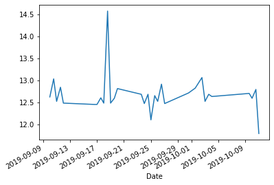
Let’s go ahead and make a plot of the distances I’ve ridden:

df['Distance'].plot.line();

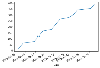
../_images/chapter9-wrangling-advanced_209_0.png

Cumulative distance might be more informative:

df['Distance'].cumsum().plot.line();

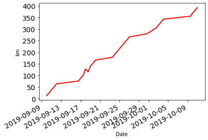
../_images/chapter9-wrangling-advanced_211_0.png

There are many configuration options for these plots which build of the matplotlib library:

df['Distance'].cumsum().plot.line(fontsize=14, linewidth = 2, color = 'r', ylabel="km");

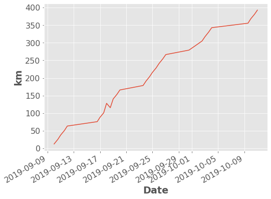
../_images/chapter9-wrangling-advanced_213_0.png

I actually usually use built-in themes for my plots which do a lot of the colour and text formatting for you:

import matplotlib.pyplot as plt
plt.style.use('ggplot')
plt.rcParams.update({'font.size': 16,
                     'axes.labelweight': 'bold',
                     'figure.figsize': (8,6)})

df['Distance'].dropna().cumsum().plot.line(ylabel="km");

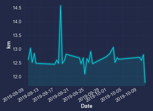
../_images/chapter9-wrangling-advanced_216_0.png

Some people have also made custom themes, like this fun cyberpunk theme:

import mplcyberpunk
plt.style.use("cyberpunk")

df['Distance'].plot.line(ylabel="km")
mplcyberpunk.add_glow_effects()

../_images/chapter9-wrangling-advanced_218_0.png

There are many other kinds of plots you can make too:

Method	Plot Type
`bar` or `barh`	bar plots
`hist`	histogram
`box`	boxplot
`kde` or `density`	density plots
`area`	area plots
`scatter`	scatter plots
`hexbin`	hexagonal bin plots
`pie`	pie plots

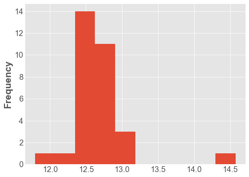
plt.style.use('ggplot')
plt.rcParams.update({'font.size': 16,
                     'axes.labelweight': 'bold',
                     'figure.figsize': (8,6)})
df['Distance'].plot.hist();

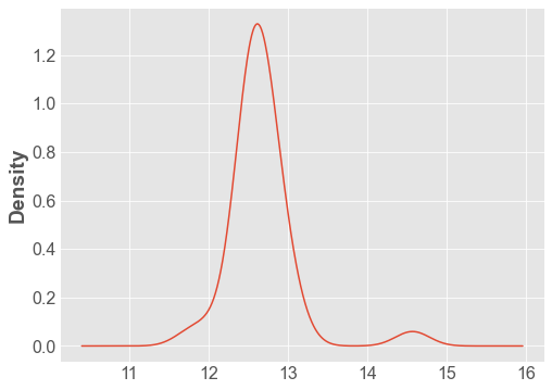
../_images/chapter9-wrangling-advanced_220_0.png

df['Distance'].plot.density();

../_images/chapter9-wrangling-advanced_221_0.png

Pandas Plotting¶

Pandas also supports a few more advanced plotting functions in the pandas.plotting module. You can view them in the Pandas documentation.

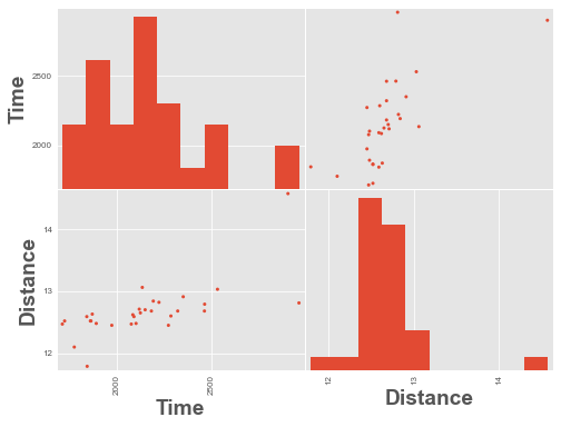
from pandas.plotting import scatter_matrix

scatter_matrix(df);

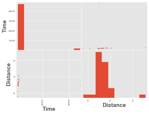
../_images/chapter9-wrangling-advanced_225_0.png

We have an outlier time in the data above, a time value of ~48,000. Let’s remove it and re-plot.

scatter_matrix(df.query('Time < 4000'), alpha=1);

../_images/chapter9-wrangling-advanced_227_0.png

5. Pandas Profiling¶

Pandas profiling is a nifty tool for generating summary reports and doing exploratory data analysis on dataframes. Pandas profiling is not part of base Pandas but you can install with:

$ conda install -c conda-forge pandas-profiling

import pandas_profiling
df = pd.read_csv('data/cycling_data.csv')
df.profile_report(progress_bar=False)