.ipynb .pdf

repository

Binder

Contents

Chapter 7: Introduction to Pandas

Chapter Outline

---

• 1. Introduction to Pandas
• 2. Pandas Series
• 3. Pandas DataFrames
• 4. Why ndarrays and Series and DataFrames?

Chapter Learning Objectives

---

• Create Pandas series with pd.Series() and Pandas dataframe with pd.DataFrame()

• Be able to access values from a Series/DataFrame by indexing, slicing and boolean indexing using notation such as df[], df.loc[], df.iloc[], df.query[]

• Perform basic arithmetic operations between two series and anticipate the result.

• Describe how Pandas assigns dtypes to Series and what the object dtype is

• Read a standard .csv file from a local path or url using Pandas pd.read_csv().

• Explain the relationship and differences between np.ndarray, pd.Series and pd.DataFrame objects in Python.

1. Introduction to Pandas

---

Pandas is most popular Python library for tabular data structures. You can think of Pandas as an extremely powerful version of Excel (but free and with a lot more features!)

Pandas can be installed using conda:

conda install pandas

We usually import pandas with the alias pd. You’ll see these two imports at the top of most data science workflows:

import pandas as pd
import numpy as np

2. Pandas Series

---

What are Series?

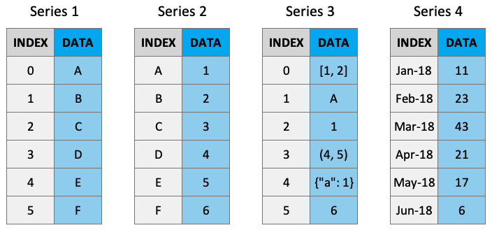
A Series is like a NumPy array but with labels. They are strictly 1-dimensional and can contain any data type (integers, strings, floats, objects, etc), including a mix of them. Series can be created from a scalar, a list, ndarray or dictionary using pd.Series() (note the captial “S”). Here are some example series:

Creating Series

By default, series are labelled with indices starting from 0. For example:

pd.Series(data = [-5, 1.3, 21, 6, 3])

0    -5.0
1     1.3
2    21.0
3     6.0
4     3.0
dtype: float64

But you can add a custom index:

pd.Series(data = [-5, 1.3, 21, 6, 3],
          index = ['a', 'b', 'c', 'd', 'e'])

a    -5.0
b     1.3
c    21.0
d     6.0
e     3.0
dtype: float64

You can create a Series from a dictionary:

pd.Series(data = {'a': 10, 'b': 20, 'c': 30})

a    10
b    20
c    30
dtype: int64

Or from an ndarray:

pd.Series(data = np.random.randn(3))

0    1.976935
1   -0.194313
2    0.173407
dtype: float64

Or even a scalar:

pd.Series(3.141)

0    3.141
dtype: float64

pd.Series(data=3.141, index=['a', 'b', 'c'])

a    3.141
b    3.141
c    3.141
dtype: float64

Series Characteristics

Series can be given a name attribute. I almost never use this but it might come up sometimes:

s = pd.Series(data = np.random.randn(5), name='random_series')
s

0   -0.655347
1   -2.245187
2    0.342516
3    0.484205
4   -1.190367
Name: random_series, dtype: float64

s.name

'random_series'

s.rename("another_name")

0   -0.655347
1   -2.245187
2    0.342516
3    0.484205
4   -1.190367
Name: another_name, dtype: float64

You can access the index labels of your series using the .index attribute:

s.index

RangeIndex(start=0, stop=5, step=1)

You can access the underlying data array using .to_numpy():

s.to_numpy()

array([-0.65534724, -2.24518664,  0.34251645,  0.48420464, -1.19036667])

pd.Series([[1, 2, 3], "b", 1]).to_numpy()

array([list([1, 2, 3]), 'b', 1], dtype=object)

Indexing and Slicing Series

Series are very much like ndarrays (in fact, series can be passed to most NumPy functions!). They can be indexed using square brackets [ ] and sliced using colon : notation:

s = pd.Series(data = range(5),
              index = ['A', 'B', 'C', 'D', 'E'])
s

A    0
B    1
C    2
D    3
E    4
dtype: int64

s[0]

0

s[[1, 2, 3]]

B    1
C    2
D    3
dtype: int64

s[0:3]

A    0
B    1
C    2
dtype: int64

Note above how array-based indexing and slicing also returns the series index.

Series are also like dictionaries, in that we can access values using index labels:

s["A"]

0

s[["B", "D", "C"]]

B    1
D    3
C    2
dtype: int64

s["A":"C"]

A    0
B    1
C    2
dtype: int64

"A" in s

True

"Z" in s

False

Series do allow for non-unique indexing, but be careful because indexing operations won’t return unique values:

x = pd.Series(data = range(5),
              index = ["A", "A", "A", "B", "C"])
x

A    0
A    1
A    2
B    3
C    4
dtype: int64

x["A"]

A    0
A    1
A    2
dtype: int64

Finally, we can also do boolean indexing with series:

s[s >= 1]

B    1
C    2
D    3
E    4
dtype: int64

s[s > s.mean()]

D    3
E    4
dtype: int64

(s != 1)

A     True
B    False
C     True
D     True
E     True
dtype: bool

Series Operations

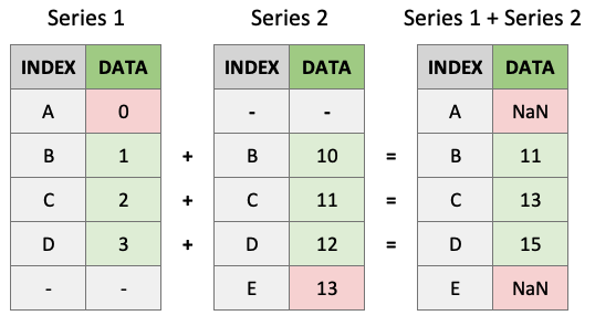
Unlike ndarrays operations between Series (+, -, /, *) align values based on their LABELS (not their position in the structure). The resulting index will be the sorted union of the two indexes. This gives you the flexibility to run operations on series regardless of their labels.

s1 = pd.Series(data = range(4),
               index = ["A", "B", "C", "D"])
s1

A    0
B    1
C    2
D    3
dtype: int64

s2 = pd.Series(data = range(10, 14),
               index = ["B", "C", "D", "E"])
s2

B    10
C    11
D    12
E    13
dtype: int64

s1 + s2

A     NaN
B    11.0
C    13.0
D    15.0
E     NaN
dtype: float64

As you can see above, indices that match will be operated on. Indices that don’t match will appear in the product but with NaN values:

We can also perform standard operations on a series, like multiplying or squaring. NumPy also accepts series as an argument to most functions because series are built off numpy arrays (more on that later):

s1 ** 2

A    0
B    1
C    4
D    9
dtype: int64

np.exp(s1)

A     1.000000
B     2.718282
C     7.389056
D    20.085537
dtype: float64

Finally, just like arrays, series have many built-in methods for various operations. You can find them all by running help(pd.Series):

print([_ for _ in dir(pd.Series) if not _.startswith("_")])  # print all common methods

['T', 'abs', 'add', 'add_prefix', 'add_suffix', 'agg', 'aggregate', 'align', 'all', 'any', 'append', 'apply', 'argmax', 'argmin', 'argsort', 'array', 'asfreq', 'asof', 'astype', 'at', 'at_time', 'attrs', 'autocorr', 'axes', 'backfill', 'between', 'between_time', 'bfill', 'bool', 'cat', 'clip', 'combine', 'combine_first', 'compare', 'convert_dtypes', 'copy', 'corr', 'count', 'cov', 'cummax', 'cummin', 'cumprod', 'cumsum', 'describe', 'diff', 'div', 'divide', 'divmod', 'dot', 'drop', 'drop_duplicates', 'droplevel', 'dropna', 'dt', 'dtype', 'dtypes', 'duplicated', 'empty', 'eq', 'equals', 'ewm', 'expanding', 'explode', 'factorize', 'ffill', 'fillna', 'filter', 'first', 'first_valid_index', 'floordiv', 'ge', 'get', 'groupby', 'gt', 'hasnans', 'head', 'hist', 'iat', 'idxmax', 'idxmin', 'iloc', 'index', 'infer_objects', 'interpolate', 'is_monotonic', 'is_monotonic_decreasing', 'is_monotonic_increasing', 'is_unique', 'isin', 'isna', 'isnull', 'item', 'items', 'iteritems', 'keys', 'kurt', 'kurtosis', 'last', 'last_valid_index', 'le', 'loc', 'lt', 'mad', 'map', 'mask', 'max', 'mean', 'median', 'memory_usage', 'min', 'mod', 'mode', 'mul', 'multiply', 'name', 'nbytes', 'ndim', 'ne', 'nlargest', 'notna', 'notnull', 'nsmallest', 'nunique', 'pad', 'pct_change', 'pipe', 'plot', 'pop', 'pow', 'prod', 'product', 'quantile', 'radd', 'rank', 'ravel', 'rdiv', 'rdivmod', 'reindex', 'reindex_like', 'rename', 'rename_axis', 'reorder_levels', 'repeat', 'replace', 'resample', 'reset_index', 'rfloordiv', 'rmod', 'rmul', 'rolling', 'round', 'rpow', 'rsub', 'rtruediv', 'sample', 'searchsorted', 'sem', 'set_axis', 'shape', 'shift', 'size', 'skew', 'slice_shift', 'sort_index', 'sort_values', 'sparse', 'squeeze', 'std', 'str', 'sub', 'subtract', 'sum', 'swapaxes', 'swaplevel', 'tail', 'take', 'to_clipboard', 'to_csv', 'to_dict', 'to_excel', 'to_frame', 'to_hdf', 'to_json', 'to_latex', 'to_list', 'to_markdown', 'to_numpy', 'to_period', 'to_pickle', 'to_sql', 'to_string', 'to_timestamp', 'to_xarray', 'tolist', 'transform', 'transpose', 'truediv', 'truncate', 'tshift', 'tz_convert', 'tz_localize', 'unique', 'unstack', 'update', 'value_counts', 'values', 'var', 'view', 'where', 'xs']

s1

A    0
B    1
C    2
D    3
dtype: int64

s1.mean()

1.5

s1.sum()

6

s1.astype(float)

A    0.0
B    1.0
C    2.0
D    3.0
dtype: float64

“Chaining” operations together is also common with pandas:

s1.add(3.141).pow(2).mean().astype(int)

22

Data Types

Series can hold all the data types (dtypes) you’re used to, e.g., int, float, bool, etc. There are a few other special data types too (object, DateTime and Categorical) which we’ll talk about in this and later chapters. You can always read more about pandas dtypes in the documentation too. For example, here’s a series of dtype int64:

x = pd.Series(range(5))
x.dtype

dtype('int64')

The dtype “object” is used for series of strings or mixed data. Pandas is currently experimenting with a dedicated string dtype StringDtype, but it is still in testing.

x = pd.Series(['A', 'B'])
x

0    A
1    B
dtype: object

x = pd.Series(['A', 1, ["I", "AM", "A", "LIST"]])
x

0                   A
1                   1
2    [I, AM, A, LIST]
dtype: object

While flexible, it is recommended to avoid the use of object dtypes because of higher memory requirements. Essentially, in an object dtype series, every single element stores information about its individual dtype. We can inspect the dtypes of all the elements in a mixed series in several ways, below I’ll use the map method:

x.map(type)

0     <class 'str'>
1     <class 'int'>
2    <class 'list'>
dtype: object

We can see that each object in our series has a different dtype. This comes at a cost. Compare the memory usage of the series below:

x1 = pd.Series([1, 2, 3])
print(f"x1 dtype: {x1.dtype}")
print(f"x1 memory usage: {x1.memory_usage(deep=True)} bytes")
print("")
x2 = pd.Series([1, 2, "3"])
print(f"x2 dtype: {x2.dtype}")
print(f"x2 memory usage: {x2.memory_usage(deep=True)} bytes")
print("")
x3 = pd.Series([1, 2, "3"]).astype('int8')  # coerce the object series to int8
print(f"x3 dtype: {x3.dtype}")
print(f"x3 memory usage: {x3.memory_usage(deep=True)} bytes")

x1 dtype: int64
x1 memory usage: 152 bytes

x2 dtype: object
x2 memory usage: 258 bytes

x3 dtype: int8
x3 memory usage: 131 bytes

In summary, try to use uniform dtypes where possible - they are more memory efficient!

One more gotcha, NaN (frequently used to represent missing values in data) is a float:

type(np.NaN)

float

This can be problematic if you have a series of integers and one missing value, because Pandas will cast the whole series to a float:

pd.Series([1, 2, 3, np.NaN])

0    1.0
1    2.0
2    3.0
3    NaN
dtype: float64

Only recently, Pandas has implemented a “nullable integer dtype”, which can handle NaN in an integer series without affecting the dtype. Note the captial “I” in the type below, differentiating it from numpy’s int64 dtype:

pd.Series([1, 2, 3, np.NaN]).astype('Int64')

0       1
1       2
2       3
3    <NA>
dtype: Int64

This is not the default in Pandas yet and functionality of this new feature is still subject to change.

3. Pandas DataFrames

---

What are DataFrames?

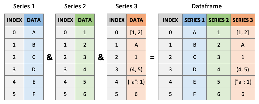
Pandas DataFrames are you’re new best friend. They are like the Excel spreadsheets you may be used to. DataFrames are really just Series stuck together! Think of a DataFrame as a dictionary of series, with the “keys” being the column labels and the “values” being the series data:

Creating DataFrames

Dataframes can be created using pd.DataFrame() (note the capital “D” and “F”). Like series, index and column labels of dataframes are labelled starting from 0 by default:

pd.DataFrame([[1, 2, 3],
              [4, 5, 6],
              [7, 8, 9]])

	0	1	2
0	1	2	3
1	4	5	6
2	7	8	9

We can use the index and columns arguments to give them labels:

pd.DataFrame([[1, 2, 3],
              [4, 5, 6],
              [7, 8, 9]],
             index = ["R1", "R2", "R3"],
             columns = ["C1", "C2", "C3"])

	C1	C2	C3
R1	1	2	3
R2	4	5	6
R3	7	8	9

There are so many ways to create dataframes. I most often create them from dictionaries or ndarrays:

pd.DataFrame({"C1": [1, 2, 3],
              "C2": ['A', 'B', 'C']},
             index=["R1", "R2", "R3"])

	C1	C2
R1	1	A
R2	2	B
R3	3	C

pd.DataFrame(np.random.randn(5, 5),
             index=[f"row_{_}" for _ in range(1, 6)],
             columns=[f"col_{_}" for _ in range(1, 6)])

	col_1	col_2	col_3	col_4	col_5
row_1	-1.867671	2.017613	-0.707579	-0.593037	-1.139370
row_2	-0.616632	0.835813	0.552254	-1.228844	-0.715589
row_3	-0.422409	-0.126844	-1.662894	-0.795743	-0.145217
row_4	-2.208804	0.492757	-2.167197	-0.511605	-0.778787
row_5	-0.302125	1.058088	0.775947	0.207029	0.204075

pd.DataFrame(np.array([['Tom', 7], ['Mike', 15], ['Tiffany', 3]]))

	0	1
0	Tom	7
1	Mike	15
2	Tiffany	3

Here’s a table of the main ways you can create dataframes (see the Pandas documentation for more):

Create DataFrame from	Code
Lists of lists	pd.DataFrame([['Tom', 7], ['Mike', 15], ['Tiffany', 3]])
ndarray	pd.DataFrame(np.array([['Tom', 7], ['Mike', 15], ['Tiffany', 3]]))
Dictionary	pd.DataFrame({"Name": ['Tom', 'Mike', 'Tiffany'], "Number": [7, 15, 3]})
List of tuples	pd.DataFrame(zip(['Tom', 'Mike', 'Tiffany'], [7, 15, 3]))
Series	pd.DataFrame({"Name": pd.Series(['Tom', 'Mike', 'Tiffany']), "Number": pd.Series([7, 15, 3])})

Indexing and Slicing DataFrames

There are several main ways to select data from a DataFrame:

1. []

2. .loc[]

3. .iloc[]

4. Boolean indexing

5. .query()

df = pd.DataFrame({"Name": ["Tom", "Mike", "Tiffany"],
                   "Language": ["Python", "Python", "R"],
                   "Courses": [5, 4, 7]})
df

	Name	Language	Courses
0	Tom	Python	5
1	Mike	Python	4
2	Tiffany	R	7

Indexing with []

Select columns by single labels, lists of labels, or slices:

df['Name']  # returns a series

0        Tom
1       Mike
2    Tiffany
Name: Name, dtype: object

df[['Name']]  # returns a dataframe!

	Name
0	Tom
1	Mike
2	Tiffany

df[['Name', 'Language']]

	Name	Language
0	Tom	Python
1	Mike	Python
2	Tiffany	R

You can only index rows by using slices, not single values (but not recommended, see preferred methods below).

df[0] # doesn't work

---------------------------------------------------------------------------
KeyError                                  Traceback (most recent call last)
/opt/miniconda3/envs/py4ds/lib/python3.8/site-packages/pandas/core/indexes/base.py in get_loc(self, key, method, tolerance)
   2897             try:
-> 2898                 return self._engine.get_loc(casted_key)
   2899             except KeyError as err:

pandas/_libs/index.pyx in pandas._libs.index.IndexEngine.get_loc()

pandas/_libs/index.pyx in pandas._libs.index.IndexEngine.get_loc()

pandas/_libs/hashtable_class_helper.pxi in pandas._libs.hashtable.PyObjectHashTable.get_item()

pandas/_libs/hashtable_class_helper.pxi in pandas._libs.hashtable.PyObjectHashTable.get_item()

KeyError: 0

The above exception was the direct cause of the following exception:

KeyError                                  Traceback (most recent call last)
<ipython-input-56-feb9bd85061b> in <module>
----> 1 df[0] # doesn't work

/opt/miniconda3/envs/py4ds/lib/python3.8/site-packages/pandas/core/frame.py in __getitem__(self, key)
   2904             if self.columns.nlevels > 1:
   2905                 return self._getitem_multilevel(key)
-> 2906             indexer = self.columns.get_loc(key)
   2907             if is_integer(indexer):
   2908                 indexer = [indexer]

/opt/miniconda3/envs/py4ds/lib/python3.8/site-packages/pandas/core/indexes/base.py in get_loc(self, key, method, tolerance)
   2898                 return self._engine.get_loc(casted_key)
   2899             except KeyError as err:
-> 2900                 raise KeyError(key) from err
   2901 
   2902         if tolerance is not None:

KeyError: 0

df[0:1] # does work

	Name	Language	Courses
0	Tom	Python	5

df[1:] # does work

	Name	Language	Courses
1	Mike	Python	4
2	Tiffany	R	7

Indexing with .loc and .iloc

Pandas created the methods .loc[] and .iloc[] as more flexible alternatives for accessing data from a dataframe. Use df.iloc[] for indexing with integers and df.loc[] for indexing with labels. These are typically the recommended methods of indexing in Pandas.

df

	Name	Language	Courses
0	Tom	Python	5
1	Mike	Python	4
2	Tiffany	R	7

First we’ll try out .iloc which accepts integers as references to rows/columns:

df.iloc[0]  # returns a series

Name           Tom
Language    Python
Courses          5
Name: 0, dtype: object

df.iloc[0:2]  # slicing returns a dataframe

	Name	Language	Courses
0	Tom	Python	5
1	Mike	Python	4

df.iloc[2, 1]  # returns the indexed object

'R'

df.iloc[[0, 1], [1, 2]]  # returns a dataframe

	Language	Courses
0	Python	5
1	Python	4

Now let’s look at .loc which accepts labels as references to rows/columns:

df.loc[:, 'Name']

0        Tom
1       Mike
2    Tiffany
Name: Name, dtype: object

df.loc[:, 'Name':'Language']

	Name	Language
0	Tom	Python
1	Mike	Python
2	Tiffany	R

df.loc[[0, 2], ['Language']]

	Language
0	Python
2	R

Sometimes we want to use a mix of integers and labels to reference data in a dataframe. The easiest way to do this is to use .loc[] with a label then use an integer in combinations with .index or .columns:

df.index

RangeIndex(start=0, stop=3, step=1)

df.columns

Index(['Name', 'Language', 'Courses'], dtype='object')

df.loc[df.index[0], 'Courses']  # I want to reference the first row and the column named "Courses"

5

df.loc[2, df.columns[1]]  # I want to reference row "2" and the second column

'R'

Boolean indexing

Just like with series, we can select data based on boolean masks:

df

	Name	Language	Courses
0	Tom	Python	5
1	Mike	Python	4
2	Tiffany	R	7

df[df['Courses'] > 5]

	Name	Language	Courses
2	Tiffany	R	7

df[df['Name'] == "Tom"]

	Name	Language	Courses
0	Tom	Python	5

Indexing with .query()

Boolean masks work fine, but I prefer to use the .query() method for selecting data. df.query() is a powerful tool for filtering data. It has an odd syntax, one of the strangest I’ve seen in Python, it is more like SQL - df.query() accepts a string expression to evaluate and it “knows” the names of the columns in your dataframe.

df.query("Courses > 4 & Language == 'Python'")

	Name	Language	Courses
0	Tom	Python	5

Note the use of single quotes AND double quotes above, lucky we have both in Python! Compare this to the equivalent boolean indexing operation and you can see that .query() is much more readable, especially as the query gets bigger!

df[(df['Courses'] > 4) & (df['Language'] == 'Python')]

	Name	Language	Courses
0	Tom	Python	5

Query also allows you to reference variable in the current workspace using the @ symbol:

course_threshold = 4
df.query("Courses > @course_threshold")

	Name	Language	Courses
0	Tom	Python	5
2	Tiffany	R	7

Indexing cheatsheet

Method	Syntax	Output
Select column	df[col_label]	Series
Select row slice	df[row_1_int:row_2_int]	DataFrame
Select row/column by label	df.loc[row_label(s), col_label(s)]	Object for single selection, Series for one row/column, otherwise DataFrame
Select row/column by integer	df.iloc[row_int(s), col_int(s)]	Object for single selection, Series for one row/column, otherwise DataFrame
Select by row integer & column label	df.loc[df.index[row_int], col_label]	Object for single selection, Series for one row/column, otherwise DataFrame
Select by row label & column integer	df.loc[row_label, df.columns[col_int]]	Object for single selection, Series for one row/column, otherwise DataFrame
Select by boolean	df[bool_vec]	Object for single selection, Series for one row/column, otherwise DataFrame
Select by boolean expression	df.query("expression")	Object for single selection, Series for one row/column, otherwise DataFrame

Reading/Writing Data From External Sources

.csv files

A lot of the time you will be loading .csv files for use in pandas. You can use the pd.read_csv() function for this. In the following chapters we’ll use a real dataset of my cycling commutes to the University of British Columbia. There are so many arguments that can be used to help read in your .csv file in an efficient and appropriate manner, feel free to check them out now (by using shift + tab in Jupyter, or typing help(pd.read_csv)).

path = 'data/cycling_data.csv'
df = pd.read_csv(path, index_col=0, parse_dates=True)
df

	Name	Type	Time	Distance	Comments
Date
2019-09-10 00:13:04	Afternoon Ride	Ride	2084	12.62	Rain
2019-09-10 13:52:18	Morning Ride	Ride	2531	13.03	rain
2019-09-11 00:23:50	Afternoon Ride	Ride	1863	12.52	Wet road but nice weather
2019-09-11 14:06:19	Morning Ride	Ride	2192	12.84	Stopped for photo of sunrise
2019-09-12 00:28:05	Afternoon Ride	Ride	1891	12.48	Tired by the end of the week
2019-09-16 13:57:48	Morning Ride	Ride	2272	12.45	Rested after the weekend!
2019-09-17 00:15:47	Afternoon Ride	Ride	1973	12.45	Legs feeling strong!
2019-09-17 13:43:34	Morning Ride	Ride	2285	12.60	Raining
2019-09-18 13:49:53	Morning Ride	Ride	2903	14.57	Raining today
2019-09-18 00:15:52	Afternoon Ride	Ride	2101	12.48	Pumped up tires
2019-09-19 00:30:01	Afternoon Ride	Ride	48062	12.48	Feeling good
2019-09-19 13:52:09	Morning Ride	Ride	2090	12.59	Getting colder which is nice
2019-09-20 01:02:05	Afternoon Ride	Ride	2961	12.81	Feeling good
2019-09-23 13:50:41	Morning Ride	Ride	2462	12.68	Rested after the weekend!
2019-09-24 00:35:42	Afternoon Ride	Ride	2076	12.47	Oiled chain, bike feels smooth
2019-09-24 13:41:24	Morning Ride	Ride	2321	12.68	Bike feeling much smoother
2019-09-25 00:07:21	Afternoon Ride	Ride	1775	12.10	Feeling really tired
2019-09-25 13:35:41	Morning Ride	Ride	2124	12.65	Stopped for photo of sunrise
2019-09-26 00:13:33	Afternoon Ride	Ride	1860	12.52	raining
2019-09-26 13:42:43	Morning Ride	Ride	2350	12.91	Detour around trucks at Jericho
2019-09-27 01:00:18	Afternoon Ride	Ride	1712	12.47	Tired by the end of the week
2019-09-30 13:53:52	Morning Ride	Ride	2118	12.71	Rested after the weekend!
2019-10-01 00:15:07	Afternoon Ride	Ride	1732	NaN	Legs feeling strong!
2019-10-01 13:45:55	Morning Ride	Ride	2222	12.82	Beautiful morning! Feeling fit
2019-10-02 00:13:09	Afternoon Ride	Ride	1756	NaN	A little tired today but good weather
2019-10-02 13:46:06	Morning Ride	Ride	2134	13.06	Bit tired today but good weather
2019-10-03 00:45:22	Afternoon Ride	Ride	1724	12.52	Feeling good
2019-10-03 13:47:36	Morning Ride	Ride	2182	12.68	Wet road
2019-10-04 01:08:08	Afternoon Ride	Ride	1870	12.63	Very tired, riding into the wind
2019-10-09 13:55:40	Morning Ride	Ride	2149	12.70	Really cold! But feeling good
2019-10-10 00:10:31	Afternoon Ride	Ride	1841	12.59	Feeling good after a holiday break!
2019-10-10 13:47:14	Morning Ride	Ride	2463	12.79	Stopped for photo of sunrise
2019-10-11 00:16:57	Afternoon Ride	Ride	1843	11.79	Bike feeling tight, needs an oil and pump

You can print a dataframe to .csv using df.to_csv(). Be sure to check out all of the possible arguments to write your dataframe exactly how you want it.

url

Pandas also facilitates reading directly from a url - pd.read_csv() accepts urls as input:

url = 'https://raw.githubusercontent.com/TomasBeuzen/toy-datasets/master/wine_1.csv'
pd.read_csv(url)

	Bottle	Grape	Origin	Alcohol	pH	Colour	Aroma
0	1	Chardonnay	Australia	14.23	3.51	White	Floral
1	2	Pinot Grigio	Italy	13.20	3.30	White	Fruity
2	3	Pinot Blanc	France	13.16	3.16	White	Citrus
3	4	Shiraz	Chile	14.91	3.39	Red	Berry
4	5	Malbec	Argentina	13.83	3.28	Red	Fruity

Other

Pandas can read data from all sorts of other file types including HTML, JSON, Excel, Parquet, Feather, etc. There are generally dedicated functions for reading these file types, see the Pandas documentation here.

Common DataFrame Operations

DataFrames have built-in functions for performing most common operations, e.g., .min(), idxmin(), sort_values(), etc. They’re all documented in the Pandas documentation here but I’ll demonstrate a few below:

df = pd.read_csv('data/cycling_data.csv')
df

	Date	Name	Type	Time	Distance	Comments
0	10 Sep 2019, 00:13:04	Afternoon Ride	Ride	2084	12.62	Rain
1	10 Sep 2019, 13:52:18	Morning Ride	Ride	2531	13.03	rain
2	11 Sep 2019, 00:23:50	Afternoon Ride	Ride	1863	12.52	Wet road but nice weather
3	11 Sep 2019, 14:06:19	Morning Ride	Ride	2192	12.84	Stopped for photo of sunrise
4	12 Sep 2019, 00:28:05	Afternoon Ride	Ride	1891	12.48	Tired by the end of the week
5	16 Sep 2019, 13:57:48	Morning Ride	Ride	2272	12.45	Rested after the weekend!
6	17 Sep 2019, 00:15:47	Afternoon Ride	Ride	1973	12.45	Legs feeling strong!
7	17 Sep 2019, 13:43:34	Morning Ride	Ride	2285	12.60	Raining
8	18 Sep 2019, 13:49:53	Morning Ride	Ride	2903	14.57	Raining today
9	18 Sep 2019, 00:15:52	Afternoon Ride	Ride	2101	12.48	Pumped up tires
10	19 Sep 2019, 00:30:01	Afternoon Ride	Ride	48062	12.48	Feeling good
11	19 Sep 2019, 13:52:09	Morning Ride	Ride	2090	12.59	Getting colder which is nice
12	20 Sep 2019, 01:02:05	Afternoon Ride	Ride	2961	12.81	Feeling good
13	23 Sep 2019, 13:50:41	Morning Ride	Ride	2462	12.68	Rested after the weekend!
14	24 Sep 2019, 00:35:42	Afternoon Ride	Ride	2076	12.47	Oiled chain, bike feels smooth
15	24 Sep 2019, 13:41:24	Morning Ride	Ride	2321	12.68	Bike feeling much smoother
16	25 Sep 2019, 00:07:21	Afternoon Ride	Ride	1775	12.10	Feeling really tired
17	25 Sep 2019, 13:35:41	Morning Ride	Ride	2124	12.65	Stopped for photo of sunrise
18	26 Sep 2019, 00:13:33	Afternoon Ride	Ride	1860	12.52	raining
19	26 Sep 2019, 13:42:43	Morning Ride	Ride	2350	12.91	Detour around trucks at Jericho
20	27 Sep 2019, 01:00:18	Afternoon Ride	Ride	1712	12.47	Tired by the end of the week
21	30 Sep 2019, 13:53:52	Morning Ride	Ride	2118	12.71	Rested after the weekend!
22	1 Oct 2019, 00:15:07	Afternoon Ride	Ride	1732	NaN	Legs feeling strong!
23	1 Oct 2019, 13:45:55	Morning Ride	Ride	2222	12.82	Beautiful morning! Feeling fit
24	2 Oct 2019, 00:13:09	Afternoon Ride	Ride	1756	NaN	A little tired today but good weather
25	2 Oct 2019, 13:46:06	Morning Ride	Ride	2134	13.06	Bit tired today but good weather
26	3 Oct 2019, 00:45:22	Afternoon Ride	Ride	1724	12.52	Feeling good
27	3 Oct 2019, 13:47:36	Morning Ride	Ride	2182	12.68	Wet road
28	4 Oct 2019, 01:08:08	Afternoon Ride	Ride	1870	12.63	Very tired, riding into the wind
29	9 Oct 2019, 13:55:40	Morning Ride	Ride	2149	12.70	Really cold! But feeling good
30	10 Oct 2019, 00:10:31	Afternoon Ride	Ride	1841	12.59	Feeling good after a holiday break!
31	10 Oct 2019, 13:47:14	Morning Ride	Ride	2463	12.79	Stopped for photo of sunrise
32	11 Oct 2019, 00:16:57	Afternoon Ride	Ride	1843	11.79	Bike feeling tight, needs an oil and pump

df.min()

Date                         1 Oct 2019, 00:15:07
Name                               Afternoon Ride
Type                                         Ride
Time                                         1712
Distance                                    11.79
Comments    A little tired today but good weather
dtype: object

df['Time'].min()

1712

df['Time'].idxmin()

20

df.iloc[20]

Date               27 Sep 2019, 01:00:18
Name                      Afternoon Ride
Type                                Ride
Time                                1712
Distance                           12.47
Comments    Tired by the end of the week
Name: 20, dtype: object

df.sum()

Date        10 Sep 2019, 00:13:0410 Sep 2019, 13:52:1811 S...
Name        Afternoon RideMorning RideAfternoon RideMornin...
Type        RideRideRideRideRideRideRideRideRideRideRideRi...
Time                                                   115922
Distance                                               392.69
Comments    RainrainWet road but nice weatherStopped for p...
dtype: object

Some methods like .mean() will only operate on numeric columns:

df.mean()

Time        3512.787879
Distance      12.667419
dtype: float64

Some methods require arguments to be specified, like .sort_values():

df.sort_values(by='Time')

	Date	Name	Type	Time	Distance	Comments
20	27 Sep 2019, 01:00:18	Afternoon Ride	Ride	1712	12.47	Tired by the end of the week
26	3 Oct 2019, 00:45:22	Afternoon Ride	Ride	1724	12.52	Feeling good
22	1 Oct 2019, 00:15:07	Afternoon Ride	Ride	1732	NaN	Legs feeling strong!
24	2 Oct 2019, 00:13:09	Afternoon Ride	Ride	1756	NaN	A little tired today but good weather
16	25 Sep 2019, 00:07:21	Afternoon Ride	Ride	1775	12.10	Feeling really tired
30	10 Oct 2019, 00:10:31	Afternoon Ride	Ride	1841	12.59	Feeling good after a holiday break!
32	11 Oct 2019, 00:16:57	Afternoon Ride	Ride	1843	11.79	Bike feeling tight, needs an oil and pump
18	26 Sep 2019, 00:13:33	Afternoon Ride	Ride	1860	12.52	raining
2	11 Sep 2019, 00:23:50	Afternoon Ride	Ride	1863	12.52	Wet road but nice weather
28	4 Oct 2019, 01:08:08	Afternoon Ride	Ride	1870	12.63	Very tired, riding into the wind
4	12 Sep 2019, 00:28:05	Afternoon Ride	Ride	1891	12.48	Tired by the end of the week
6	17 Sep 2019, 00:15:47	Afternoon Ride	Ride	1973	12.45	Legs feeling strong!
14	24 Sep 2019, 00:35:42	Afternoon Ride	Ride	2076	12.47	Oiled chain, bike feels smooth
0	10 Sep 2019, 00:13:04	Afternoon Ride	Ride	2084	12.62	Rain
11	19 Sep 2019, 13:52:09	Morning Ride	Ride	2090	12.59	Getting colder which is nice
9	18 Sep 2019, 00:15:52	Afternoon Ride	Ride	2101	12.48	Pumped up tires
21	30 Sep 2019, 13:53:52	Morning Ride	Ride	2118	12.71	Rested after the weekend!
17	25 Sep 2019, 13:35:41	Morning Ride	Ride	2124	12.65	Stopped for photo of sunrise
25	2 Oct 2019, 13:46:06	Morning Ride	Ride	2134	13.06	Bit tired today but good weather
29	9 Oct 2019, 13:55:40	Morning Ride	Ride	2149	12.70	Really cold! But feeling good
27	3 Oct 2019, 13:47:36	Morning Ride	Ride	2182	12.68	Wet road
3	11 Sep 2019, 14:06:19	Morning Ride	Ride	2192	12.84	Stopped for photo of sunrise
23	1 Oct 2019, 13:45:55	Morning Ride	Ride	2222	12.82	Beautiful morning! Feeling fit
5	16 Sep 2019, 13:57:48	Morning Ride	Ride	2272	12.45	Rested after the weekend!
7	17 Sep 2019, 13:43:34	Morning Ride	Ride	2285	12.60	Raining
15	24 Sep 2019, 13:41:24	Morning Ride	Ride	2321	12.68	Bike feeling much smoother
19	26 Sep 2019, 13:42:43	Morning Ride	Ride	2350	12.91	Detour around trucks at Jericho
13	23 Sep 2019, 13:50:41	Morning Ride	Ride	2462	12.68	Rested after the weekend!
31	10 Oct 2019, 13:47:14	Morning Ride	Ride	2463	12.79	Stopped for photo of sunrise
1	10 Sep 2019, 13:52:18	Morning Ride	Ride	2531	13.03	rain
8	18 Sep 2019, 13:49:53	Morning Ride	Ride	2903	14.57	Raining today
12	20 Sep 2019, 01:02:05	Afternoon Ride	Ride	2961	12.81	Feeling good
10	19 Sep 2019, 00:30:01	Afternoon Ride	Ride	48062	12.48	Feeling good

df.sort_values(by='Time', ascending=False)

	Date	Name	Type	Time	Distance	Comments
10	19 Sep 2019, 00:30:01	Afternoon Ride	Ride	48062	12.48	Feeling good
12	20 Sep 2019, 01:02:05	Afternoon Ride	Ride	2961	12.81	Feeling good
8	18 Sep 2019, 13:49:53	Morning Ride	Ride	2903	14.57	Raining today
1	10 Sep 2019, 13:52:18	Morning Ride	Ride	2531	13.03	rain
31	10 Oct 2019, 13:47:14	Morning Ride	Ride	2463	12.79	Stopped for photo of sunrise
13	23 Sep 2019, 13:50:41	Morning Ride	Ride	2462	12.68	Rested after the weekend!
19	26 Sep 2019, 13:42:43	Morning Ride	Ride	2350	12.91	Detour around trucks at Jericho
15	24 Sep 2019, 13:41:24	Morning Ride	Ride	2321	12.68	Bike feeling much smoother
7	17 Sep 2019, 13:43:34	Morning Ride	Ride	2285	12.60	Raining
5	16 Sep 2019, 13:57:48	Morning Ride	Ride	2272	12.45	Rested after the weekend!
23	1 Oct 2019, 13:45:55	Morning Ride	Ride	2222	12.82	Beautiful morning! Feeling fit
3	11 Sep 2019, 14:06:19	Morning Ride	Ride	2192	12.84	Stopped for photo of sunrise
27	3 Oct 2019, 13:47:36	Morning Ride	Ride	2182	12.68	Wet road
29	9 Oct 2019, 13:55:40	Morning Ride	Ride	2149	12.70	Really cold! But feeling good
25	2 Oct 2019, 13:46:06	Morning Ride	Ride	2134	13.06	Bit tired today but good weather
17	25 Sep 2019, 13:35:41	Morning Ride	Ride	2124	12.65	Stopped for photo of sunrise
21	30 Sep 2019, 13:53:52	Morning Ride	Ride	2118	12.71	Rested after the weekend!
9	18 Sep 2019, 00:15:52	Afternoon Ride	Ride	2101	12.48	Pumped up tires
11	19 Sep 2019, 13:52:09	Morning Ride	Ride	2090	12.59	Getting colder which is nice
0	10 Sep 2019, 00:13:04	Afternoon Ride	Ride	2084	12.62	Rain
14	24 Sep 2019, 00:35:42	Afternoon Ride	Ride	2076	12.47	Oiled chain, bike feels smooth
6	17 Sep 2019, 00:15:47	Afternoon Ride	Ride	1973	12.45	Legs feeling strong!
4	12 Sep 2019, 00:28:05	Afternoon Ride	Ride	1891	12.48	Tired by the end of the week
28	4 Oct 2019, 01:08:08	Afternoon Ride	Ride	1870	12.63	Very tired, riding into the wind
2	11 Sep 2019, 00:23:50	Afternoon Ride	Ride	1863	12.52	Wet road but nice weather
18	26 Sep 2019, 00:13:33	Afternoon Ride	Ride	1860	12.52	raining
32	11 Oct 2019, 00:16:57	Afternoon Ride	Ride	1843	11.79	Bike feeling tight, needs an oil and pump
30	10 Oct 2019, 00:10:31	Afternoon Ride	Ride	1841	12.59	Feeling good after a holiday break!
16	25 Sep 2019, 00:07:21	Afternoon Ride	Ride	1775	12.10	Feeling really tired
24	2 Oct 2019, 00:13:09	Afternoon Ride	Ride	1756	NaN	A little tired today but good weather
22	1 Oct 2019, 00:15:07	Afternoon Ride	Ride	1732	NaN	Legs feeling strong!
26	3 Oct 2019, 00:45:22	Afternoon Ride	Ride	1724	12.52	Feeling good
20	27 Sep 2019, 01:00:18	Afternoon Ride	Ride	1712	12.47	Tired by the end of the week

Some methods will operate on the index/columns, like .sort_index():

df.sort_index(ascending=False)

	Date	Name	Type	Time	Distance	Comments
32	11 Oct 2019, 00:16:57	Afternoon Ride	Ride	1843	11.79	Bike feeling tight, needs an oil and pump
31	10 Oct 2019, 13:47:14	Morning Ride	Ride	2463	12.79	Stopped for photo of sunrise
30	10 Oct 2019, 00:10:31	Afternoon Ride	Ride	1841	12.59	Feeling good after a holiday break!
29	9 Oct 2019, 13:55:40	Morning Ride	Ride	2149	12.70	Really cold! But feeling good
28	4 Oct 2019, 01:08:08	Afternoon Ride	Ride	1870	12.63	Very tired, riding into the wind
27	3 Oct 2019, 13:47:36	Morning Ride	Ride	2182	12.68	Wet road
26	3 Oct 2019, 00:45:22	Afternoon Ride	Ride	1724	12.52	Feeling good
25	2 Oct 2019, 13:46:06	Morning Ride	Ride	2134	13.06	Bit tired today but good weather
24	2 Oct 2019, 00:13:09	Afternoon Ride	Ride	1756	NaN	A little tired today but good weather
23	1 Oct 2019, 13:45:55	Morning Ride	Ride	2222	12.82	Beautiful morning! Feeling fit
22	1 Oct 2019, 00:15:07	Afternoon Ride	Ride	1732	NaN	Legs feeling strong!
21	30 Sep 2019, 13:53:52	Morning Ride	Ride	2118	12.71	Rested after the weekend!
20	27 Sep 2019, 01:00:18	Afternoon Ride	Ride	1712	12.47	Tired by the end of the week
19	26 Sep 2019, 13:42:43	Morning Ride	Ride	2350	12.91	Detour around trucks at Jericho
18	26 Sep 2019, 00:13:33	Afternoon Ride	Ride	1860	12.52	raining
17	25 Sep 2019, 13:35:41	Morning Ride	Ride	2124	12.65	Stopped for photo of sunrise
16	25 Sep 2019, 00:07:21	Afternoon Ride	Ride	1775	12.10	Feeling really tired
15	24 Sep 2019, 13:41:24	Morning Ride	Ride	2321	12.68	Bike feeling much smoother
14	24 Sep 2019, 00:35:42	Afternoon Ride	Ride	2076	12.47	Oiled chain, bike feels smooth
13	23 Sep 2019, 13:50:41	Morning Ride	Ride	2462	12.68	Rested after the weekend!
12	20 Sep 2019, 01:02:05	Afternoon Ride	Ride	2961	12.81	Feeling good
11	19 Sep 2019, 13:52:09	Morning Ride	Ride	2090	12.59	Getting colder which is nice
10	19 Sep 2019, 00:30:01	Afternoon Ride	Ride	48062	12.48	Feeling good
9	18 Sep 2019, 00:15:52	Afternoon Ride	Ride	2101	12.48	Pumped up tires
8	18 Sep 2019, 13:49:53	Morning Ride	Ride	2903	14.57	Raining today
7	17 Sep 2019, 13:43:34	Morning Ride	Ride	2285	12.60	Raining
6	17 Sep 2019, 00:15:47	Afternoon Ride	Ride	1973	12.45	Legs feeling strong!
5	16 Sep 2019, 13:57:48	Morning Ride	Ride	2272	12.45	Rested after the weekend!
4	12 Sep 2019, 00:28:05	Afternoon Ride	Ride	1891	12.48	Tired by the end of the week
3	11 Sep 2019, 14:06:19	Morning Ride	Ride	2192	12.84	Stopped for photo of sunrise
2	11 Sep 2019, 00:23:50	Afternoon Ride	Ride	1863	12.52	Wet road but nice weather
1	10 Sep 2019, 13:52:18	Morning Ride	Ride	2531	13.03	rain
0	10 Sep 2019, 00:13:04	Afternoon Ride	Ride	2084	12.62	Rain

4. Why ndarrays and Series and DataFrames?

At this point, you might be asking why we need all these different data structures. Well, they all serve different purposes and are suited to different tasks. For example:

• NumPy is typically faster/uses less memory than Pandas;

• not all Python packages are compatible with NumPy & Pandas;

• the ability to add labels to data can be useful (e.g., for time series);

• NumPy and Pandas have different built-in functions available.

My advice: use the simplest data structure that fulfills your needs!

Finally, we’ve seen how to go from: ndarray (np.array()) -> series (pd.series()) -> dataframe (pd.DataFrame()). Remember that we can also go the other way: dataframe/series -> ndarray using df.to_numpy().

Chapter 6: NumPy Implementation Details Chapter 8: Basic Data Wrangling With Pandas