Chapter 8: Basic Data Wrangling With Pandas
Chapter Outline
Chapter Learning Objectives
Inspect a dataframe with
df.head(),df.tail(),df.info(),df.describe().Obtain dataframe summaries with
df.info()anddf.describe().Manipulate how a dataframe displays in Jupyter by modifying Pandas configuration options such as
pd.set_option("display.max_rows", n).Rename columns of a dataframe using the
df.rename()function or by accessing thedf.columnsattribute.Modify the index name and index values of a dataframe using
.set_index(),.reset_index(),df.index.name,.index.Use
df.melt()anddf.pivot()to reshape dataframes, specifically to make tidy dataframes.Combine dataframes using
df.merge()andpd.concat()and know when to use these different methods.Apply functions to a dataframe
df.apply()anddf.applymap()Perform grouping and aggregating operations using
df.groupby()anddf.agg().Perform aggregating methods on grouped or ungrouped objects such as finding the minimum, maximum and sum of values in a dataframe using
df.agg().Remove or fill missing values in a dataframe with
df.dropna()anddf.fillna().
1. DataFrame Characteristics
Last chapter we looked at how we can create dataframes. Let’s now look at some helpful ways we can view our dataframe.
import numpy as np
import pandas as pd
Head/Tail
The .head() and .tail() methods allow you to view the top/bottom n (default 5) rows of a dataframe. Let’s load in the cycling data set from last chapter and try them out:
df = pd.read_csv('data/cycling_data.csv')
df.head()
| Date | Name | Type | Time | Distance | Comments | |
|---|---|---|---|---|---|---|
| 0 | 10 Sep 2019, 00:13:04 | Afternoon Ride | Ride | 2084 | 12.62 | Rain |
| 1 | 10 Sep 2019, 13:52:18 | Morning Ride | Ride | 2531 | 13.03 | rain |
| 2 | 11 Sep 2019, 00:23:50 | Afternoon Ride | Ride | 1863 | 12.52 | Wet road but nice weather |
| 3 | 11 Sep 2019, 14:06:19 | Morning Ride | Ride | 2192 | 12.84 | Stopped for photo of sunrise |
| 4 | 12 Sep 2019, 00:28:05 | Afternoon Ride | Ride | 1891 | 12.48 | Tired by the end of the week |
The default return value is 5 rows, but we can pass in any number we like. For example, let’s take a look at the top 10 rows:
df.head(10)
| Date | Name | Type | Time | Distance | Comments | |
|---|---|---|---|---|---|---|
| 0 | 10 Sep 2019, 00:13:04 | Afternoon Ride | Ride | 2084 | 12.62 | Rain |
| 1 | 10 Sep 2019, 13:52:18 | Morning Ride | Ride | 2531 | 13.03 | rain |
| 2 | 11 Sep 2019, 00:23:50 | Afternoon Ride | Ride | 1863 | 12.52 | Wet road but nice weather |
| 3 | 11 Sep 2019, 14:06:19 | Morning Ride | Ride | 2192 | 12.84 | Stopped for photo of sunrise |
| 4 | 12 Sep 2019, 00:28:05 | Afternoon Ride | Ride | 1891 | 12.48 | Tired by the end of the week |
| 5 | 16 Sep 2019, 13:57:48 | Morning Ride | Ride | 2272 | 12.45 | Rested after the weekend! |
| 6 | 17 Sep 2019, 00:15:47 | Afternoon Ride | Ride | 1973 | 12.45 | Legs feeling strong! |
| 7 | 17 Sep 2019, 13:43:34 | Morning Ride | Ride | 2285 | 12.60 | Raining |
| 8 | 18 Sep 2019, 13:49:53 | Morning Ride | Ride | 2903 | 14.57 | Raining today |
| 9 | 18 Sep 2019, 00:15:52 | Afternoon Ride | Ride | 2101 | 12.48 | Pumped up tires |
Or the bottom 5 rows:
df.tail()
| Date | Name | Type | Time | Distance | Comments | |
|---|---|---|---|---|---|---|
| 28 | 4 Oct 2019, 01:08:08 | Afternoon Ride | Ride | 1870 | 12.63 | Very tired, riding into the wind |
| 29 | 9 Oct 2019, 13:55:40 | Morning Ride | Ride | 2149 | 12.70 | Really cold! But feeling good |
| 30 | 10 Oct 2019, 00:10:31 | Afternoon Ride | Ride | 1841 | 12.59 | Feeling good after a holiday break! |
| 31 | 10 Oct 2019, 13:47:14 | Morning Ride | Ride | 2463 | 12.79 | Stopped for photo of sunrise |
| 32 | 11 Oct 2019, 00:16:57 | Afternoon Ride | Ride | 1843 | 11.79 | Bike feeling tight, needs an oil and pump |
DataFrame Summaries
Three very helpful attributes/functions for getting high-level summaries of your dataframe are:
.shape.info().describe()
.shape is just like the ndarray attribute we’ve seen previously. It gives the shape (rows, cols) of your dataframe:
df.shape
(33, 6)
.info() prints information about the dataframe itself, such as dtypes, memory usages, non-null values, etc:
df.info()
<class 'pandas.core.frame.DataFrame'>
RangeIndex: 33 entries, 0 to 32
Data columns (total 6 columns):
 #   Column    Non-Null Count  Dtype
---  ------    --------------  -----
 0   Date      33 non-null     object
 1   Name      33 non-null     object
 2   Type      33 non-null     object
 3   Time      33 non-null     int64
 4   Distance  31 non-null     float64
 5   Comments  33 non-null     object
dtypes: float64(1), int64(1), object(4)
memory usage: 1.7+ KB
.describe() provides summary statistics of the values within a dataframe:
df.describe()
| Time | Distance | |
|---|---|---|
| count | 33.000000 | 31.000000 |
| mean | 3512.787879 | 12.667419 |
| std | 8003.309233 | 0.428618 |
| min | 1712.000000 | 11.790000 |
| 25% | 1863.000000 | 12.480000 |
| 50% | 2118.000000 | 12.620000 |
| 75% | 2285.000000 | 12.750000 |
| max | 48062.000000 | 14.570000 |
By default, .describe() only print summaries of numeric features. We can force it to give summaries on all features using the argument include='all' (although they may not make sense!):
df.describe(include='all')
| Date | Name | Type | Time | Distance | Comments | |
|---|---|---|---|---|---|---|
| count | 33 | 33 | 33 | 33.000000 | 31.000000 | 33 |
| unique | 33 | 2 | 1 | NaN | NaN | 25 |
| top | 17 Sep 2019, 00:15:47 | Afternoon Ride | Ride | NaN | NaN | Feeling good |
| freq | 1 | 17 | 33 | NaN | NaN | 3 |
| mean | NaN | NaN | NaN | 3512.787879 | 12.667419 | NaN |
| std | NaN | NaN | NaN | 8003.309233 | 0.428618 | NaN |
| min | NaN | NaN | NaN | 1712.000000 | 11.790000 | NaN |
| 25% | NaN | NaN | NaN | 1863.000000 | 12.480000 | NaN |
| 50% | NaN | NaN | NaN | 2118.000000 | 12.620000 | NaN |
| 75% | NaN | NaN | NaN | 2285.000000 | 12.750000 | NaN |
| max | NaN | NaN | NaN | 48062.000000 | 14.570000 | NaN |
Displaying DataFrames
Displaying your dataframes effectively can be an important part of your workflow. If a dataframe has more than 60 rows, Pandas will only display the first 5 and last 5 rows:
pd.DataFrame(np.random.rand(100))
| 0 | |
|---|---|
| 0 | 0.150874 |
| 1 | 0.799918 |
| 2 | 0.387415 |
| 3 | 0.508148 |
| 4 | 0.965465 |
| ... | ... |
| 95 | 0.411632 |
| 96 | 0.325456 |
| 97 | 0.874201 |
| 98 | 0.617720 |
| 99 | 0.084849 |
100 rows × 1 columns
For dataframes of less than 60 rows, Pandas will print the whole dataframe:
df
| Date | Name | Type | Time | Distance | Comments | |
|---|---|---|---|---|---|---|
| 0 | 10 Sep 2019, 00:13:04 | Afternoon Ride | Ride | 2084 | 12.62 | Rain |
| 1 | 10 Sep 2019, 13:52:18 | Morning Ride | Ride | 2531 | 13.03 | rain |
| 2 | 11 Sep 2019, 00:23:50 | Afternoon Ride | Ride | 1863 | 12.52 | Wet road but nice weather |
| 3 | 11 Sep 2019, 14:06:19 | Morning Ride | Ride | 2192 | 12.84 | Stopped for photo of sunrise |
| 4 | 12 Sep 2019, 00:28:05 | Afternoon Ride | Ride | 1891 | 12.48 | Tired by the end of the week |
| 5 | 16 Sep 2019, 13:57:48 | Morning Ride | Ride | 2272 | 12.45 | Rested after the weekend! |
| 6 | 17 Sep 2019, 00:15:47 | Afternoon Ride | Ride | 1973 | 12.45 | Legs feeling strong! |
| 7 | 17 Sep 2019, 13:43:34 | Morning Ride | Ride | 2285 | 12.60 | Raining |
| 8 | 18 Sep 2019, 13:49:53 | Morning Ride | Ride | 2903 | 14.57 | Raining today |
| 9 | 18 Sep 2019, 00:15:52 | Afternoon Ride | Ride | 2101 | 12.48 | Pumped up tires |
| 10 | 19 Sep 2019, 00:30:01 | Afternoon Ride | Ride | 48062 | 12.48 | Feeling good |
| 11 | 19 Sep 2019, 13:52:09 | Morning Ride | Ride | 2090 | 12.59 | Getting colder which is nice |
| 12 | 20 Sep 2019, 01:02:05 | Afternoon Ride | Ride | 2961 | 12.81 | Feeling good |
| 13 | 23 Sep 2019, 13:50:41 | Morning Ride | Ride | 2462 | 12.68 | Rested after the weekend! |
| 14 | 24 Sep 2019, 00:35:42 | Afternoon Ride | Ride | 2076 | 12.47 | Oiled chain, bike feels smooth |
| 15 | 24 Sep 2019, 13:41:24 | Morning Ride | Ride | 2321 | 12.68 | Bike feeling much smoother |
| 16 | 25 Sep 2019, 00:07:21 | Afternoon Ride | Ride | 1775 | 12.10 | Feeling really tired |
| 17 | 25 Sep 2019, 13:35:41 | Morning Ride | Ride | 2124 | 12.65 | Stopped for photo of sunrise |
| 18 | 26 Sep 2019, 00:13:33 | Afternoon Ride | Ride | 1860 | 12.52 | raining |
| 19 | 26 Sep 2019, 13:42:43 | Morning Ride | Ride | 2350 | 12.91 | Detour around trucks at Jericho |
| 20 | 27 Sep 2019, 01:00:18 | Afternoon Ride | Ride | 1712 | 12.47 | Tired by the end of the week |
| 21 | 30 Sep 2019, 13:53:52 | Morning Ride | Ride | 2118 | 12.71 | Rested after the weekend! |
| 22 | 1 Oct 2019, 00:15:07 | Afternoon Ride | Ride | 1732 | NaN | Legs feeling strong! |
| 23 | 1 Oct 2019, 13:45:55 | Morning Ride | Ride | 2222 | 12.82 | Beautiful morning! Feeling fit |
| 24 | 2 Oct 2019, 00:13:09 | Afternoon Ride | Ride | 1756 | NaN | A little tired today but good weather |
| 25 | 2 Oct 2019, 13:46:06 | Morning Ride | Ride | 2134 | 13.06 | Bit tired today but good weather |
| 26 | 3 Oct 2019, 00:45:22 | Afternoon Ride | Ride | 1724 | 12.52 | Feeling good |
| 27 | 3 Oct 2019, 13:47:36 | Morning Ride | Ride | 2182 | 12.68 | Wet road |
| 28 | 4 Oct 2019, 01:08:08 | Afternoon Ride | Ride | 1870 | 12.63 | Very tired, riding into the wind |
| 29 | 9 Oct 2019, 13:55:40 | Morning Ride | Ride | 2149 | 12.70 | Really cold! But feeling good |
| 30 | 10 Oct 2019, 00:10:31 | Afternoon Ride | Ride | 1841 | 12.59 | Feeling good after a holiday break! |
| 31 | 10 Oct 2019, 13:47:14 | Morning Ride | Ride | 2463 | 12.79 | Stopped for photo of sunrise |
| 32 | 11 Oct 2019, 00:16:57 | Afternoon Ride | Ride | 1843 | 11.79 | Bike feeling tight, needs an oil and pump |
I find the 60 row threshold to be a little too much, I prefer something more like 20. You can change the setting using pd.set_option("display.max_rows", 20) so that anything with more than 20 rows will be summarised by the first and last 5 rows as before:
pd.set_option("display.max_rows", 20)
df
| Date | Name | Type | Time | Distance | Comments | |
|---|---|---|---|---|---|---|
| 0 | 10 Sep 2019, 00:13:04 | Afternoon Ride | Ride | 2084 | 12.62 | Rain |
| 1 | 10 Sep 2019, 13:52:18 | Morning Ride | Ride | 2531 | 13.03 | rain |
| 2 | 11 Sep 2019, 00:23:50 | Afternoon Ride | Ride | 1863 | 12.52 | Wet road but nice weather |
| 3 | 11 Sep 2019, 14:06:19 | Morning Ride | Ride | 2192 | 12.84 | Stopped for photo of sunrise |
| 4 | 12 Sep 2019, 00:28:05 | Afternoon Ride | Ride | 1891 | 12.48 | Tired by the end of the week |
| ... | ... | ... | ... | ... | ... | ... |
| 28 | 4 Oct 2019, 01:08:08 | Afternoon Ride | Ride | 1870 | 12.63 | Very tired, riding into the wind |
| 29 | 9 Oct 2019, 13:55:40 | Morning Ride | Ride | 2149 | 12.70 | Really cold! But feeling good |
| 30 | 10 Oct 2019, 00:10:31 | Afternoon Ride | Ride | 1841 | 12.59 | Feeling good after a holiday break! |
| 31 | 10 Oct 2019, 13:47:14 | Morning Ride | Ride | 2463 | 12.79 | Stopped for photo of sunrise |
| 32 | 11 Oct 2019, 00:16:57 | Afternoon Ride | Ride | 1843 | 11.79 | Bike feeling tight, needs an oil and pump |
33 rows × 6 columns
There are also other display options you can change, such as how many columns are shown, how numbers are formatted, etc. See the official documentation for more.
One display option I will point out is that Pandas allows you to style your tables, for example by highlighting negative values, or adding conditional colour maps to your dataframe. Below I’ll style values based on their value ranging from negative (purple) to postive (yellow) but you can see the styling documentation for more examples.
test = pd.DataFrame(np.random.randn(5, 5),
                    index = [f"row_{_}" for _ in range(5)],
                    columns = [f"feature_{_}" for _ in range(5)])
test.style.background_gradient(cmap='plasma')
| feature_0 | feature_1 | feature_2 | feature_3 | feature_4 | |
|---|---|---|---|---|---|
| row_0 | -0.908801 | -1.349283 | 0.587406 | 0.086509 | 0.479789 |
| row_1 | 2.119295 | -0.372110 | 0.443444 | 0.551942 | -0.511610 |
| row_2 | 0.030793 | -0.454157 | 0.439636 | 0.948702 | -0.604266 |
| row_3 | -0.264686 | -1.371427 | 1.311990 | 0.365076 | 0.466767 |
| row_4 | 0.231278 | 2.009801 | 0.586166 | -1.307132 | -1.425747 |
Views vs Copies
In previous chapters we’ve discussed views (“looking” at a part of an existing object) and copies (making a new copy of the object in memory). These things get a little abstract with Pandas and “…it’s very hard to predict whether it will return a view or a copy” (that’s a quote straight from a dedicated section in the Pandas documentation).
Basically, it depends on the operation you are trying to perform, your dataframe’s structure and the memory layout of the underlying array. But don’t worry, let me tell you all you need to know. Firstly, the most common warning you’ll encounter in Pandas is the SettingWithCopy, Pandas raises it as a warning that you might not be doing what you think you’re doing. Let’s see an example. You may recall there is one outlier Time in our dataframe:
df[df['Time'] > 4000]
| Date | Name | Type | Time | Distance | Comments | |
|---|---|---|---|---|---|---|
| 10 | 19 Sep 2019, 00:30:01 | Afternoon Ride | Ride | 48062 | 12.48 | Feeling good |
Imagine we wanted to change this to 2000. You’d probably do the following:
df[df['Time'] > 4000]['Time'] = 2000
/opt/miniconda3/envs/mds511/lib/python3.7/site-packages/ipykernel_launcher.py:1: SettingWithCopyWarning:
A value is trying to be set on a copy of a slice from a DataFrame.
Try using .loc[row_indexer,col_indexer] = value instead

See the caveats in the documentation: https://pandas.pydata.org/pandas-docs/stable/user_guide/indexing.html#returning-a-view-versus-a-copy
  """Entry point for launching an IPython kernel.
Ah, there’s that warning. Did our dataframe get changed?
df[df['Time'] > 4000]
| Date | Name | Type | Time | Distance | Comments | |
|---|---|---|---|---|---|---|
| 10 | 19 Sep 2019, 00:30:01 | Afternoon Ride | Ride | 48062 | 12.48 | Feeling good |
No it didn’t, even though you probably thought it did. What happened above is that df[df['Time'] > 4000] was executed first and returned a copy of the dataframe, we can confirm by using id():
print(f"The id of the original dataframe is: {id(df)}")
print(f" The id of the indexed dataframe is: {id(df[df['Time'] > 4000])}")
The id of the original dataframe is: 4588085840
 The id of the indexed dataframe is: 4612421712
We then tried to set a value on this new object by appending ['Time'] = 2000. Pandas is warning us that we are doing that operation on a copy of the original dataframe, which is probably not what we want. To fix this, you need to index in a single go, using .loc[] for example:
df.loc[df['Time'] > 4000, 'Time'] = 2000
No error this time! And let’s confirm the change:
df[df['Time'] > 4000]
| Date | Name | Type | Time | Distance | Comments |
|---|
The second thing you need to know is that if you’re ever in doubt about whether something is a view or a copy, you can just use the .copy() method to force a copy of a dataframe. Just like this:
df2 = df[df['Time'] > 4000].copy()
That way, your guaranteed a copy that you can modify as you wish.
2. Basic DataFrame Manipulations
Renaming Columns
We can rename columns two ways:
Using
.rename()(to selectively change column names)By setting the
.columnsattribute (to change all column names at once)
df
| Date | Name | Type | Time | Distance | Comments | |
|---|---|---|---|---|---|---|
| 0 | 10 Sep 2019, 00:13:04 | Afternoon Ride | Ride | 2084 | 12.62 | Rain |
| 1 | 10 Sep 2019, 13:52:18 | Morning Ride | Ride | 2531 | 13.03 | rain |
| 2 | 11 Sep 2019, 00:23:50 | Afternoon Ride | Ride | 1863 | 12.52 | Wet road but nice weather |
| 3 | 11 Sep 2019, 14:06:19 | Morning Ride | Ride | 2192 | 12.84 | Stopped for photo of sunrise |
| 4 | 12 Sep 2019, 00:28:05 | Afternoon Ride | Ride | 1891 | 12.48 | Tired by the end of the week |
| ... | ... | ... | ... | ... | ... | ... |
| 28 | 4 Oct 2019, 01:08:08 | Afternoon Ride | Ride | 1870 | 12.63 | Very tired, riding into the wind |
| 29 | 9 Oct 2019, 13:55:40 | Morning Ride | Ride | 2149 | 12.70 | Really cold! But feeling good |
| 30 | 10 Oct 2019, 00:10:31 | Afternoon Ride | Ride | 1841 | 12.59 | Feeling good after a holiday break! |
| 31 | 10 Oct 2019, 13:47:14 | Morning Ride | Ride | 2463 | 12.79 | Stopped for photo of sunrise |
| 32 | 11 Oct 2019, 00:16:57 | Afternoon Ride | Ride | 1843 | 11.79 | Bike feeling tight, needs an oil and pump |
33 rows × 6 columns
Let’s give it a go:
df.rename(columns={"Date": "Datetime",
                   "Comments": "Notes"})
df
| Date | Name | Type | Time | Distance | Comments | |
|---|---|---|---|---|---|---|
| 0 | 10 Sep 2019, 00:13:04 | Afternoon Ride | Ride | 2084 | 12.62 | Rain |
| 1 | 10 Sep 2019, 13:52:18 | Morning Ride | Ride | 2531 | 13.03 | rain |
| 2 | 11 Sep 2019, 00:23:50 | Afternoon Ride | Ride | 1863 | 12.52 | Wet road but nice weather |
| 3 | 11 Sep 2019, 14:06:19 | Morning Ride | Ride | 2192 | 12.84 | Stopped for photo of sunrise |
| 4 | 12 Sep 2019, 00:28:05 | Afternoon Ride | Ride | 1891 | 12.48 | Tired by the end of the week |
| ... | ... | ... | ... | ... | ... | ... |
| 28 | 4 Oct 2019, 01:08:08 | Afternoon Ride | Ride | 1870 | 12.63 | Very tired, riding into the wind |
| 29 | 9 Oct 2019, 13:55:40 | Morning Ride | Ride | 2149 | 12.70 | Really cold! But feeling good |
| 30 | 10 Oct 2019, 00:10:31 | Afternoon Ride | Ride | 1841 | 12.59 | Feeling good after a holiday break! |
| 31 | 10 Oct 2019, 13:47:14 | Morning Ride | Ride | 2463 | 12.79 | Stopped for photo of sunrise |
| 32 | 11 Oct 2019, 00:16:57 | Afternoon Ride | Ride | 1843 | 11.79 | Bike feeling tight, needs an oil and pump |
33 rows × 6 columns
Wait? What happened? Nothing changed? In the code above we did actually rename columns of our dataframe but we didn’t modify the dataframe inplace, we made a copy of it. There are generally two options for making permanent dataframe changes:
Use the argument
inplace=True, e.g.,df.rename(..., inplace=True), available in most functions/methods
Re-assign, e.g.,
df = df.rename(...)The Pandas team recommends Method 2 (re-assign), for a few reasons (mostly to do with how memory is allocated under the hood).
df = df.rename(columns={"Date": "Datetime",
                        "Comments": "Notes"})
df
| Datetime | Name | Type | Time | Distance | Notes | |
|---|---|---|---|---|---|---|
| 0 | 10 Sep 2019, 00:13:04 | Afternoon Ride | Ride | 2084 | 12.62 | Rain |
| 1 | 10 Sep 2019, 13:52:18 | Morning Ride | Ride | 2531 | 13.03 | rain |
| 2 | 11 Sep 2019, 00:23:50 | Afternoon Ride | Ride | 1863 | 12.52 | Wet road but nice weather |
| 3 | 11 Sep 2019, 14:06:19 | Morning Ride | Ride | 2192 | 12.84 | Stopped for photo of sunrise |
| 4 | 12 Sep 2019, 00:28:05 | Afternoon Ride | Ride | 1891 | 12.48 | Tired by the end of the week |
| ... | ... | ... | ... | ... | ... | ... |
| 28 | 4 Oct 2019, 01:08:08 | Afternoon Ride | Ride | 1870 | 12.63 | Very tired, riding into the wind |
| 29 | 9 Oct 2019, 13:55:40 | Morning Ride | Ride | 2149 | 12.70 | Really cold! But feeling good |
| 30 | 10 Oct 2019, 00:10:31 | Afternoon Ride | Ride | 1841 | 12.59 | Feeling good after a holiday break! |
| 31 | 10 Oct 2019, 13:47:14 | Morning Ride | Ride | 2463 | 12.79 | Stopped for photo of sunrise |
| 32 | 11 Oct 2019, 00:16:57 | Afternoon Ride | Ride | 1843 | 11.79 | Bike feeling tight, needs an oil and pump |
33 rows × 6 columns
If you wish to change all of the columns of a dataframe, you can do so by setting the .columns attribute:
df.columns = [f"Column {_}" for _ in range(1, 7)]
df
| Column 1 | Column 2 | Column 3 | Column 4 | Column 5 | Column 6 | |
|---|---|---|---|---|---|---|
| 0 | 10 Sep 2019, 00:13:04 | Afternoon Ride | Ride | 2084 | 12.62 | Rain |
| 1 | 10 Sep 2019, 13:52:18 | Morning Ride | Ride | 2531 | 13.03 | rain |
| 2 | 11 Sep 2019, 00:23:50 | Afternoon Ride | Ride | 1863 | 12.52 | Wet road but nice weather |
| 3 | 11 Sep 2019, 14:06:19 | Morning Ride | Ride | 2192 | 12.84 | Stopped for photo of sunrise |
| 4 | 12 Sep 2019, 00:28:05 | Afternoon Ride | Ride | 1891 | 12.48 | Tired by the end of the week |
| ... | ... | ... | ... | ... | ... | ... |
| 28 | 4 Oct 2019, 01:08:08 | Afternoon Ride | Ride | 1870 | 12.63 | Very tired, riding into the wind |
| 29 | 9 Oct 2019, 13:55:40 | Morning Ride | Ride | 2149 | 12.70 | Really cold! But feeling good |
| 30 | 10 Oct 2019, 00:10:31 | Afternoon Ride | Ride | 1841 | 12.59 | Feeling good after a holiday break! |
| 31 | 10 Oct 2019, 13:47:14 | Morning Ride | Ride | 2463 | 12.79 | Stopped for photo of sunrise |
| 32 | 11 Oct 2019, 00:16:57 | Afternoon Ride | Ride | 1843 | 11.79 | Bike feeling tight, needs an oil and pump |
33 rows × 6 columns
Changing the Index
You can change the index labels of a dataframe in 3 main ways:
.set_index()to make one of the columns of the dataframe the indexDirectly modify
df.index.nameto change the index name.reset_index()to move the current index as a column and to reset the index with integer labels starting from 0Directly modify the
.index()attribute
df
| Column 1 | Column 2 | Column 3 | Column 4 | Column 5 | Column 6 | |
|---|---|---|---|---|---|---|
| 0 | 10 Sep 2019, 00:13:04 | Afternoon Ride | Ride | 2084 | 12.62 | Rain |
| 1 | 10 Sep 2019, 13:52:18 | Morning Ride | Ride | 2531 | 13.03 | rain |
| 2 | 11 Sep 2019, 00:23:50 | Afternoon Ride | Ride | 1863 | 12.52 | Wet road but nice weather |
| 3 | 11 Sep 2019, 14:06:19 | Morning Ride | Ride | 2192 | 12.84 | Stopped for photo of sunrise |
| 4 | 12 Sep 2019, 00:28:05 | Afternoon Ride | Ride | 1891 | 12.48 | Tired by the end of the week |
| ... | ... | ... | ... | ... | ... | ... |
| 28 | 4 Oct 2019, 01:08:08 | Afternoon Ride | Ride | 1870 | 12.63 | Very tired, riding into the wind |
| 29 | 9 Oct 2019, 13:55:40 | Morning Ride | Ride | 2149 | 12.70 | Really cold! But feeling good |
| 30 | 10 Oct 2019, 00:10:31 | Afternoon Ride | Ride | 1841 | 12.59 | Feeling good after a holiday break! |
| 31 | 10 Oct 2019, 13:47:14 | Morning Ride | Ride | 2463 | 12.79 | Stopped for photo of sunrise |
| 32 | 11 Oct 2019, 00:16:57 | Afternoon Ride | Ride | 1843 | 11.79 | Bike feeling tight, needs an oil and pump |
33 rows × 6 columns
Below I will set the index as Column 1 and rename the index to “New Index”:
df = df.set_index("Column 1")
df.index.name = "New Index"
df
| Column 2 | Column 3 | Column 4 | Column 5 | Column 6 | |
|---|---|---|---|---|---|
| New Index | |||||
| 10 Sep 2019, 00:13:04 | Afternoon Ride | Ride | 2084 | 12.62 | Rain |
| 10 Sep 2019, 13:52:18 | Morning Ride | Ride | 2531 | 13.03 | rain |
| 11 Sep 2019, 00:23:50 | Afternoon Ride | Ride | 1863 | 12.52 | Wet road but nice weather |
| 11 Sep 2019, 14:06:19 | Morning Ride | Ride | 2192 | 12.84 | Stopped for photo of sunrise |
| 12 Sep 2019, 00:28:05 | Afternoon Ride | Ride | 1891 | 12.48 | Tired by the end of the week |
| ... | ... | ... | ... | ... | ... |
| 4 Oct 2019, 01:08:08 | Afternoon Ride | Ride | 1870 | 12.63 | Very tired, riding into the wind |
| 9 Oct 2019, 13:55:40 | Morning Ride | Ride | 2149 | 12.70 | Really cold! But feeling good |
| 10 Oct 2019, 00:10:31 | Afternoon Ride | Ride | 1841 | 12.59 | Feeling good after a holiday break! |
| 10 Oct 2019, 13:47:14 | Morning Ride | Ride | 2463 | 12.79 | Stopped for photo of sunrise |
| 11 Oct 2019, 00:16:57 | Afternoon Ride | Ride | 1843 | 11.79 | Bike feeling tight, needs an oil and pump |
33 rows × 5 columns
I can send the index back to a column and have a default integer index using .reset_index():
df = df.reset_index()
df
| New Index | Column 2 | Column 3 | Column 4 | Column 5 | Column 6 | |
|---|---|---|---|---|---|---|
| 0 | 10 Sep 2019, 00:13:04 | Afternoon Ride | Ride | 2084 | 12.62 | Rain |
| 1 | 10 Sep 2019, 13:52:18 | Morning Ride | Ride | 2531 | 13.03 | rain |
| 2 | 11 Sep 2019, 00:23:50 | Afternoon Ride | Ride | 1863 | 12.52 | Wet road but nice weather |
| 3 | 11 Sep 2019, 14:06:19 | Morning Ride | Ride | 2192 | 12.84 | Stopped for photo of sunrise |
| 4 | 12 Sep 2019, 00:28:05 | Afternoon Ride | Ride | 1891 | 12.48 | Tired by the end of the week |
| ... | ... | ... | ... | ... | ... | ... |
| 28 | 4 Oct 2019, 01:08:08 | Afternoon Ride | Ride | 1870 | 12.63 | Very tired, riding into the wind |
| 29 | 9 Oct 2019, 13:55:40 | Morning Ride | Ride | 2149 | 12.70 | Really cold! But feeling good |
| 30 | 10 Oct 2019, 00:10:31 | Afternoon Ride | Ride | 1841 | 12.59 | Feeling good after a holiday break! |
| 31 | 10 Oct 2019, 13:47:14 | Morning Ride | Ride | 2463 | 12.79 | Stopped for photo of sunrise |
| 32 | 11 Oct 2019, 00:16:57 | Afternoon Ride | Ride | 1843 | 11.79 | Bike feeling tight, needs an oil and pump |
33 rows × 6 columns
Like with column names, we can also modify the index directly, but I can’t remember ever doing this, usually I’ll use .set_index():
df.index
RangeIndex(start=0, stop=33, step=1)
df.index = range(100, 133, 1)
df
| New Index | Column 2 | Column 3 | Column 4 | Column 5 | Column 6 | |
|---|---|---|---|---|---|---|
| 100 | 10 Sep 2019, 00:13:04 | Afternoon Ride | Ride | 2084 | 12.62 | Rain |
| 101 | 10 Sep 2019, 13:52:18 | Morning Ride | Ride | 2531 | 13.03 | rain |
| 102 | 11 Sep 2019, 00:23:50 | Afternoon Ride | Ride | 1863 | 12.52 | Wet road but nice weather |
| 103 | 11 Sep 2019, 14:06:19 | Morning Ride | Ride | 2192 | 12.84 | Stopped for photo of sunrise |
| 104 | 12 Sep 2019, 00:28:05 | Afternoon Ride | Ride | 1891 | 12.48 | Tired by the end of the week |
| ... | ... | ... | ... | ... | ... | ... |
| 128 | 4 Oct 2019, 01:08:08 | Afternoon Ride | Ride | 1870 | 12.63 | Very tired, riding into the wind |
| 129 | 9 Oct 2019, 13:55:40 | Morning Ride | Ride | 2149 | 12.70 | Really cold! But feeling good |
| 130 | 10 Oct 2019, 00:10:31 | Afternoon Ride | Ride | 1841 | 12.59 | Feeling good after a holiday break! |
| 131 | 10 Oct 2019, 13:47:14 | Morning Ride | Ride | 2463 | 12.79 | Stopped for photo of sunrise |
| 132 | 11 Oct 2019, 00:16:57 | Afternoon Ride | Ride | 1843 | 11.79 | Bike feeling tight, needs an oil and pump |
33 rows × 6 columns
Adding/Removing Columns
There are two main ways to add/remove columns of a dataframe:
Use
[]to add columnsUse
.drop()to drop columns
Let’s re-read in a fresh copy of the cycling dataset.
df = pd.read_csv('data/cycling_data.csv')
df
| Date | Name | Type | Time | Distance | Comments | |
|---|---|---|---|---|---|---|
| 0 | 10 Sep 2019, 00:13:04 | Afternoon Ride | Ride | 2084 | 12.62 | Rain |
| 1 | 10 Sep 2019, 13:52:18 | Morning Ride | Ride | 2531 | 13.03 | rain |
| 2 | 11 Sep 2019, 00:23:50 | Afternoon Ride | Ride | 1863 | 12.52 | Wet road but nice weather |
| 3 | 11 Sep 2019, 14:06:19 | Morning Ride | Ride | 2192 | 12.84 | Stopped for photo of sunrise |
| 4 | 12 Sep 2019, 00:28:05 | Afternoon Ride | Ride | 1891 | 12.48 | Tired by the end of the week |
| ... | ... | ... | ... | ... | ... | ... |
| 28 | 4 Oct 2019, 01:08:08 | Afternoon Ride | Ride | 1870 | 12.63 | Very tired, riding into the wind |
| 29 | 9 Oct 2019, 13:55:40 | Morning Ride | Ride | 2149 | 12.70 | Really cold! But feeling good |
| 30 | 10 Oct 2019, 00:10:31 | Afternoon Ride | Ride | 1841 | 12.59 | Feeling good after a holiday break! |
| 31 | 10 Oct 2019, 13:47:14 | Morning Ride | Ride | 2463 | 12.79 | Stopped for photo of sunrise |
| 32 | 11 Oct 2019, 00:16:57 | Afternoon Ride | Ride | 1843 | 11.79 | Bike feeling tight, needs an oil and pump |
33 rows × 6 columns
We can add a new column to a dataframe by simply using [] with a new column name and value(s):
df['Rider'] = 'Tom Beuzen'
df['Avg Speed'] = df['Distance'] * 1000 / df['Time']  # avg. speed in m/s
df
| Date | Name | Type | Time | Distance | Comments | Rider | Avg Speed | |
|---|---|---|---|---|---|---|---|---|
| 0 | 10 Sep 2019, 00:13:04 | Afternoon Ride | Ride | 2084 | 12.62 | Rain | Tom Beuzen | 6.055662 |
| 1 | 10 Sep 2019, 13:52:18 | Morning Ride | Ride | 2531 | 13.03 | rain | Tom Beuzen | 5.148163 |
| 2 | 11 Sep 2019, 00:23:50 | Afternoon Ride | Ride | 1863 | 12.52 | Wet road but nice weather | Tom Beuzen | 6.720344 |
| 3 | 11 Sep 2019, 14:06:19 | Morning Ride | Ride | 2192 | 12.84 | Stopped for photo of sunrise | Tom Beuzen | 5.857664 |
| 4 | 12 Sep 2019, 00:28:05 | Afternoon Ride | Ride | 1891 | 12.48 | Tired by the end of the week | Tom Beuzen | 6.599683 |
| ... | ... | ... | ... | ... | ... | ... | ... | ... |
| 28 | 4 Oct 2019, 01:08:08 | Afternoon Ride | Ride | 1870 | 12.63 | Very tired, riding into the wind | Tom Beuzen | 6.754011 |
| 29 | 9 Oct 2019, 13:55:40 | Morning Ride | Ride | 2149 | 12.70 | Really cold! But feeling good | Tom Beuzen | 5.909725 |
| 30 | 10 Oct 2019, 00:10:31 | Afternoon Ride | Ride | 1841 | 12.59 | Feeling good after a holiday break! | Tom Beuzen | 6.838675 |
| 31 | 10 Oct 2019, 13:47:14 | Morning Ride | Ride | 2463 | 12.79 | Stopped for photo of sunrise | Tom Beuzen | 5.192854 |
| 32 | 11 Oct 2019, 00:16:57 | Afternoon Ride | Ride | 1843 | 11.79 | Bike feeling tight, needs an oil and pump | Tom Beuzen | 6.397179 |
33 rows × 8 columns
df = df.drop(columns=['Rider', 'Avg Speed'])
df
| Date | Name | Type | Time | Distance | Comments | |
|---|---|---|---|---|---|---|
| 0 | 10 Sep 2019, 00:13:04 | Afternoon Ride | Ride | 2084 | 12.62 | Rain |
| 1 | 10 Sep 2019, 13:52:18 | Morning Ride | Ride | 2531 | 13.03 | rain |
| 2 | 11 Sep 2019, 00:23:50 | Afternoon Ride | Ride | 1863 | 12.52 | Wet road but nice weather |
| 3 | 11 Sep 2019, 14:06:19 | Morning Ride | Ride | 2192 | 12.84 | Stopped for photo of sunrise |
| 4 | 12 Sep 2019, 00:28:05 | Afternoon Ride | Ride | 1891 | 12.48 | Tired by the end of the week |
| ... | ... | ... | ... | ... | ... | ... |
| 28 | 4 Oct 2019, 01:08:08 | Afternoon Ride | Ride | 1870 | 12.63 | Very tired, riding into the wind |
| 29 | 9 Oct 2019, 13:55:40 | Morning Ride | Ride | 2149 | 12.70 | Really cold! But feeling good |
| 30 | 10 Oct 2019, 00:10:31 | Afternoon Ride | Ride | 1841 | 12.59 | Feeling good after a holiday break! |
| 31 | 10 Oct 2019, 13:47:14 | Morning Ride | Ride | 2463 | 12.79 | Stopped for photo of sunrise |
| 32 | 11 Oct 2019, 00:16:57 | Afternoon Ride | Ride | 1843 | 11.79 | Bike feeling tight, needs an oil and pump |
33 rows × 6 columns
Adding/Removing Rows
You won’t often be adding rows to a dataframe manually (you’ll usually add rows through concatenating/joining - that’s coming up next). You can add/remove rows of a dataframe in two ways:
Use
.append()to add rowsUse
.drop()to drop rows
df
| Date | Name | Type | Time | Distance | Comments | |
|---|---|---|---|---|---|---|
| 0 | 10 Sep 2019, 00:13:04 | Afternoon Ride | Ride | 2084 | 12.62 | Rain |
| 1 | 10 Sep 2019, 13:52:18 | Morning Ride | Ride | 2531 | 13.03 | rain |
| 2 | 11 Sep 2019, 00:23:50 | Afternoon Ride | Ride | 1863 | 12.52 | Wet road but nice weather |
| 3 | 11 Sep 2019, 14:06:19 | Morning Ride | Ride | 2192 | 12.84 | Stopped for photo of sunrise |
| 4 | 12 Sep 2019, 00:28:05 | Afternoon Ride | Ride | 1891 | 12.48 | Tired by the end of the week |
| ... | ... | ... | ... | ... | ... | ... |
| 28 | 4 Oct 2019, 01:08:08 | Afternoon Ride | Ride | 1870 | 12.63 | Very tired, riding into the wind |
| 29 | 9 Oct 2019, 13:55:40 | Morning Ride | Ride | 2149 | 12.70 | Really cold! But feeling good |
| 30 | 10 Oct 2019, 00:10:31 | Afternoon Ride | Ride | 1841 | 12.59 | Feeling good after a holiday break! |
| 31 | 10 Oct 2019, 13:47:14 | Morning Ride | Ride | 2463 | 12.79 | Stopped for photo of sunrise |
| 32 | 11 Oct 2019, 00:16:57 | Afternoon Ride | Ride | 1843 | 11.79 | Bike feeling tight, needs an oil and pump |
33 rows × 6 columns
Let’s add a new row to the bottom of this dataframe:
another_row = pd.DataFrame([["12 Oct 2019, 00:10:57", "Morning Ride", "Ride",
                             2331, 12.67, "Washed and oiled bike last night"]],
                           columns = df.columns,
                           index = [33])
df = df.append(another_row)
df
| Date | Name | Type | Time | Distance | Comments | |
|---|---|---|---|---|---|---|
| 0 | 10 Sep 2019, 00:13:04 | Afternoon Ride | Ride | 2084 | 12.62 | Rain |
| 1 | 10 Sep 2019, 13:52:18 | Morning Ride | Ride | 2531 | 13.03 | rain |
| 2 | 11 Sep 2019, 00:23:50 | Afternoon Ride | Ride | 1863 | 12.52 | Wet road but nice weather |
| 3 | 11 Sep 2019, 14:06:19 | Morning Ride | Ride | 2192 | 12.84 | Stopped for photo of sunrise |
| 4 | 12 Sep 2019, 00:28:05 | Afternoon Ride | Ride | 1891 | 12.48 | Tired by the end of the week |
| ... | ... | ... | ... | ... | ... | ... |
| 29 | 9 Oct 2019, 13:55:40 | Morning Ride | Ride | 2149 | 12.70 | Really cold! But feeling good |
| 30 | 10 Oct 2019, 00:10:31 | Afternoon Ride | Ride | 1841 | 12.59 | Feeling good after a holiday break! |
| 31 | 10 Oct 2019, 13:47:14 | Morning Ride | Ride | 2463 | 12.79 | Stopped for photo of sunrise |
| 32 | 11 Oct 2019, 00:16:57 | Afternoon Ride | Ride | 1843 | 11.79 | Bike feeling tight, needs an oil and pump |
| 33 | 12 Oct 2019, 00:10:57 | Morning Ride | Ride | 2331 | 12.67 | Washed and oiled bike last night |
34 rows × 6 columns
We can drop all rows above index 30 using .drop():
df.drop(index=range(30, 34))
| Date | Name | Type | Time | Distance | Comments | |
|---|---|---|---|---|---|---|
| 0 | 10 Sep 2019, 00:13:04 | Afternoon Ride | Ride | 2084 | 12.62 | Rain |
| 1 | 10 Sep 2019, 13:52:18 | Morning Ride | Ride | 2531 | 13.03 | rain |
| 2 | 11 Sep 2019, 00:23:50 | Afternoon Ride | Ride | 1863 | 12.52 | Wet road but nice weather |
| 3 | 11 Sep 2019, 14:06:19 | Morning Ride | Ride | 2192 | 12.84 | Stopped for photo of sunrise |
| 4 | 12 Sep 2019, 00:28:05 | Afternoon Ride | Ride | 1891 | 12.48 | Tired by the end of the week |
| ... | ... | ... | ... | ... | ... | ... |
| 25 | 2 Oct 2019, 13:46:06 | Morning Ride | Ride | 2134 | 13.06 | Bit tired today but good weather |
| 26 | 3 Oct 2019, 00:45:22 | Afternoon Ride | Ride | 1724 | 12.52 | Feeling good |
| 27 | 3 Oct 2019, 13:47:36 | Morning Ride | Ride | 2182 | 12.68 | Wet road |
| 28 | 4 Oct 2019, 01:08:08 | Afternoon Ride | Ride | 1870 | 12.63 | Very tired, riding into the wind |
| 29 | 9 Oct 2019, 13:55:40 | Morning Ride | Ride | 2149 | 12.70 | Really cold! But feeling good |
30 rows × 6 columns
3. DataFrame Reshaping
Tidy data is about “linking the structure of a dataset with its semantics (its meaning)”. It is defined by:
Each variable forms a column
Each observation forms a row
Each type of observational unit forms a table
Often you’ll need to reshape a dataframe to make it tidy (or for some other purpose).
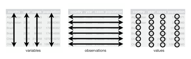
Source: r4ds
Melt and Pivot
Pandas .melt(), .pivot() and .pivot_table() can help reshape dataframes
.melt(): make wide data long..pivot(): make long data width..pivot_table(): same as.pivot()but can handle multiple indexes.
Source: Garrick Aden-Buie’s GitHub
The below data shows how many courses different instructors taught across different years. If the question you want to answer is something like: “Does the number of courses taught vary depending on year?” then the below would probably not be considered tidy because there are multiple observations of courses taught in a year per row (i.e., there is data for 2018, 2019 and 2020 in a single row):
df = pd.DataFrame({"Name": ["Tom", "Mike", "Tiffany", "Varada", "Joel"],
                   "2018": [1, 3, 4, 5, 3],
                   "2019": [2, 4, 3, 2, 1],
                   "2020": [5, 2, 4, 4, 3]})
df
| Name | 2018 | 2019 | 2020 | |
|---|---|---|---|---|
| 0 | Tom | 1 | 2 | 5 |
| 1 | Mike | 3 | 4 | 2 |
| 2 | Tiffany | 4 | 3 | 4 |
| 3 | Varada | 5 | 2 | 4 |
| 4 | Joel | 3 | 1 | 3 |
Let’s make it tidy with .melt(). .melt() takes a few arguments, most important is the id_vars which indicated which column should be the “identifier”.
df_melt = df.melt(id_vars="Name",
                  var_name="Year",
                  value_name="Courses")
df_melt
| Name | Year | Courses | |
|---|---|---|---|
| 0 | Tom | 2018 | 1 |
| 1 | Mike | 2018 | 3 |
| 2 | Tiffany | 2018 | 4 |
| 3 | Varada | 2018 | 5 |
| 4 | Joel | 2018 | 3 |
| 5 | Tom | 2019 | 2 |
| 6 | Mike | 2019 | 4 |
| 7 | Tiffany | 2019 | 3 |
| 8 | Varada | 2019 | 2 |
| 9 | Joel | 2019 | 1 |
| 10 | Tom | 2020 | 5 |
| 11 | Mike | 2020 | 2 |
| 12 | Tiffany | 2020 | 4 |
| 13 | Varada | 2020 | 4 |
| 14 | Joel | 2020 | 3 |
The value_vars argument allows us to select which specific variables we want to “melt” (if you don’t specify value_vars, all non-identifier columns will be used). For example, below I’m omitting the 2018 column:
df.melt(id_vars="Name",
        value_vars=["2019", "2020"],
        var_name="Year",
        value_name="Courses")
| Name | Year | Courses | |
|---|---|---|---|
| 0 | Tom | 2019 | 2 |
| 1 | Mike | 2019 | 4 |
| 2 | Tiffany | 2019 | 3 |
| 3 | Varada | 2019 | 2 |
| 4 | Joel | 2019 | 1 |
| 5 | Tom | 2020 | 5 |
| 6 | Mike | 2020 | 2 |
| 7 | Tiffany | 2020 | 4 |
| 8 | Varada | 2020 | 4 |
| 9 | Joel | 2020 | 3 |
Sometimes, you want to make long data wide, which we can do with .pivot(). When using .pivot() we need to specify the index to pivot on, and the columns that will be used to make the new columns of the wider dataframe:
df_pivot = df_melt.pivot(index="Name",
                         columns="Year",
                         values="Courses")
df_pivot
| Year | 2018 | 2019 | 2020 |
|---|---|---|---|
| Name | |||
| Joel | 3 | 1 | 3 |
| Mike | 3 | 4 | 2 |
| Tiffany | 4 | 3 | 4 |
| Tom | 1 | 2 | 5 |
| Varada | 5 | 2 | 4 |
You’ll notice that Pandas set our specified index as the index of the new dataframe and preserved the label of the columns. We can easily remove these names and reset the index to make our dataframe look like it originally did:
df_pivot = df_pivot.reset_index()
df_pivot.columns.name = None
df_pivot
| Name | 2018 | 2019 | 2020 | |
|---|---|---|---|---|
| 0 | Joel | 3 | 1 | 3 |
| 1 | Mike | 3 | 4 | 2 |
| 2 | Tiffany | 4 | 3 | 4 |
| 3 | Tom | 1 | 2 | 5 |
| 4 | Varada | 5 | 2 | 4 |
.pivot() will often get you what you want, but it won’t work if you want to:
Use multiple indexes (next chapter), or
Have duplicate index/column labels
In these cases you’ll have to use .pivot_table(). I won’t focus on it too much here because I’d rather you learn about pivot() first.
df = pd.DataFrame({"Name": ["Tom", "Tom", "Mike", "Mike"],
                   "Department": ["CS", "STATS", "CS", "STATS"],
                   "2018": [1, 2, 3, 1],
                   "2019": [2, 3, 4, 2],
                   "2020": [5, 1, 2, 2]}).melt(id_vars=["Name", "Department"], var_name="Year", value_name="Courses")
df
| Name | Department | Year | Courses | |
|---|---|---|---|---|
| 0 | Tom | CS | 2018 | 1 |
| 1 | Tom | STATS | 2018 | 2 |
| 2 | Mike | CS | 2018 | 3 |
| 3 | Mike | STATS | 2018 | 1 |
| 4 | Tom | CS | 2019 | 2 |
| 5 | Tom | STATS | 2019 | 3 |
| 6 | Mike | CS | 2019 | 4 |
| 7 | Mike | STATS | 2019 | 2 |
| 8 | Tom | CS | 2020 | 5 |
| 9 | Tom | STATS | 2020 | 1 |
| 10 | Mike | CS | 2020 | 2 |
| 11 | Mike | STATS | 2020 | 2 |
In the above case, we have duplicates in Name, so pivot() won’t work. It will throw us a ValueError: Index contains duplicate entries, cannot reshape:
df.pivot(index="Name",
         columns="Year",
         values="Courses")
---------------------------------------------------------------------------
ValueError                                Traceback (most recent call last)
<ipython-input-41-585e29950052> in <module>
      1 df.pivot(index="Name",
      2          columns="Year",
----> 3          values="Courses")

/opt/miniconda3/envs/mds511/lib/python3.7/site-packages/pandas/core/frame.py in pivot(self, index, columns, values)
   6665         from pandas.core.reshape.pivot import pivot
   6666
-> 6667         return pivot(self, index=index, columns=columns, values=values)
   6668
   6669     _shared_docs[

/opt/miniconda3/envs/mds511/lib/python3.7/site-packages/pandas/core/reshape/pivot.py in pivot(data, index, columns, values)
    475         else:
    476             indexed = data._constructor_sliced(data[values]._values, index=index)
--> 477     return indexed.unstack(columns)
    478
    479

/opt/miniconda3/envs/mds511/lib/python3.7/site-packages/pandas/core/series.py in unstack(self, level, fill_value)
   3888         from pandas.core.reshape.reshape import unstack
   3889
-> 3890         return unstack(self, level, fill_value)
   3891
   3892     # ----------------------------------------------------------------------

/opt/miniconda3/envs/mds511/lib/python3.7/site-packages/pandas/core/reshape/reshape.py in unstack(obj, level, fill_value)
    423             return _unstack_extension_series(obj, level, fill_value)
    424         unstacker = _Unstacker(
--> 425             obj.index, level=level, constructor=obj._constructor_expanddim,
    426         )
    427         return unstacker.get_result(

/opt/miniconda3/envs/mds511/lib/python3.7/site-packages/pandas/core/reshape/reshape.py in __init__(self, index, level, constructor)
    118             raise ValueError("Unstacked DataFrame is too big, causing int32 overflow")
    119
--> 120         self._make_selectors()
    121
    122     @cache_readonly

/opt/miniconda3/envs/mds511/lib/python3.7/site-packages/pandas/core/reshape/reshape.py in _make_selectors(self)
    167
    168         if mask.sum() < len(self.index):
--> 169             raise ValueError("Index contains duplicate entries, cannot reshape")
    170
    171         self.group_index = comp_index

ValueError: Index contains duplicate entries, cannot reshape
In such a case, we’d use .pivot_table(). It will apply an aggregation function to our duplicates, in this case, we’ll sum() them up:
df.pivot_table(index="Name", columns='Year', values='Courses', aggfunc='sum')
| Year | 2018 | 2019 | 2020 |
|---|---|---|---|
| Name | |||
| Mike | 4 | 6 | 4 |
| Tom | 3 | 5 | 6 |
If we wanted to keep the numbers per department, we could specify both Name and Department as multiple indexes:
df.pivot_table(index=["Name", "Department"], columns='Year', values='Courses')
| Year | 2018 | 2019 | 2020 | |
|---|---|---|---|---|
| Name | Department | |||
| Mike | CS | 3 | 4 | 2 |
| STATS | 1 | 2 | 2 | |
| Tom | CS | 1 | 2 | 5 |
| STATS | 2 | 3 | 1 |
The result above is a mutlti-index or “hierarchically indexed” dataframe (more on those next chapter). If you ever have a need to use it, you can read more about pivot_table() in the documentation.
4. Working with Multiple DataFrames
Often you’ll work with multiple dataframes that you want to stick together or merge. df.merge() and df.concat() are all you need to know for combining dataframes. The Pandas documentation is very helpful for these functions, but they are pretty easy to grasp.
Note
The example joins shown in this section are inspired by Chapter 15 of Jenny Bryan’s STAT 545 materials.
Sticking DataFrames Together with pd.concat()
You can use pd.concat() to stick dataframes together:
Vertically: if they have the same columns, OR
Horizontally: if they have the same rows
df1 = pd.DataFrame({'A': [1, 3, 5],
                    'B': [2, 4, 6]})
df2 = pd.DataFrame({'A': [7, 9, 11],
                    'B': [8, 10, 12]})
df1
| A | B | |
|---|---|---|
| 0 | 1 | 2 |
| 1 | 3 | 4 |
| 2 | 5 | 6 |
df2
| A | B | |
|---|---|---|
| 0 | 7 | 8 |
| 1 | 9 | 10 |
| 2 | 11 | 12 |
pd.concat((df1, df2), axis=0) # axis=0 specifies a vertical stick, i.e., on the columns
| A | B | |
|---|---|---|
| 0 | 1 | 2 |
| 1 | 3 | 4 |
| 2 | 5 | 6 |
| 0 | 7 | 8 |
| 1 | 9 | 10 |
| 2 | 11 | 12 |
Notice that the indexes were simply joined together? This may or may not be what you want. To reset the index, you can specify the argument ignore_index=True:
pd.concat((df1, df2), axis=0, ignore_index=True)
| A | B | |
|---|---|---|
| 0 | 1 | 2 |
| 1 | 3 | 4 |
| 2 | 5 | 6 |
| 3 | 7 | 8 |
| 4 | 9 | 10 |
| 5 | 11 | 12 |
Use axis=1 to stick together horizontally:
pd.concat((df1, df2), axis=1, ignore_index=True)
| 0 | 1 | 2 | 3 | |
|---|---|---|---|---|
| 0 | 1 | 2 | 7 | 8 |
| 1 | 3 | 4 | 9 | 10 |
| 2 | 5 | 6 | 11 | 12 |
You are not limited to just two dataframes, you can concatenate as many as you want:
pd.concat((df1, df2, df1, df2), axis=0, ignore_index=True)
| A | B | |
|---|---|---|
| 0 | 1 | 2 |
| 1 | 3 | 4 |
| 2 | 5 | 6 |
| 3 | 7 | 8 |
| 4 | 9 | 10 |
| 5 | 11 | 12 |
| 6 | 1 | 2 |
| 7 | 3 | 4 |
| 8 | 5 | 6 |
| 9 | 7 | 8 |
| 10 | 9 | 10 |
| 11 | 11 | 12 |
Joining DataFrames with pd.merge()
pd.merge() gives you the ability to “join” dataframes using different rules (just like with SQL if you’re familiar with it). You can use df.merge() to join dataframes based on shared key columns. Methods include:
“inner join”
“outer join”
“left join”
“right join”
See this great cheat sheet and these great animations for more insights.
df1 = pd.DataFrame({"name": ['Magneto', 'Storm', 'Mystique', 'Batman', 'Joker', 'Catwoman', 'Hellboy'],
                    'alignment': ['bad', 'good', 'bad', 'good', 'bad', 'bad', 'good'],
                    'gender': ['male', 'female', 'female', 'male', 'male', 'female', 'male'],
                    'publisher': ['Marvel', 'Marvel', 'Marvel', 'DC', 'DC', 'DC', 'Dark Horse Comics']})
df2 = pd.DataFrame({'publisher': ['DC', 'Marvel', 'Image'],
                    'year_founded': [1934, 1939, 1992]})
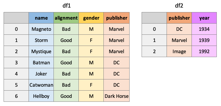
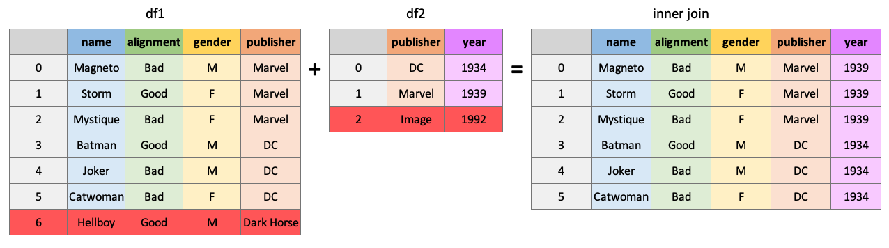
An “inner” join will return all rows of df1 where matching values for “publisher” are found in df2:
pd.merge(df1, df2, how="inner", on="publisher")
| name | alignment | gender | publisher | year_founded | |
|---|---|---|---|---|---|
| 0 | Magneto | bad | male | Marvel | 1939 |
| 1 | Storm | good | female | Marvel | 1939 |
| 2 | Mystique | bad | female | Marvel | 1939 |
| 3 | Batman | good | male | DC | 1934 |
| 4 | Joker | bad | male | DC | 1934 |
| 5 | Catwoman | bad | female | DC | 1934 |
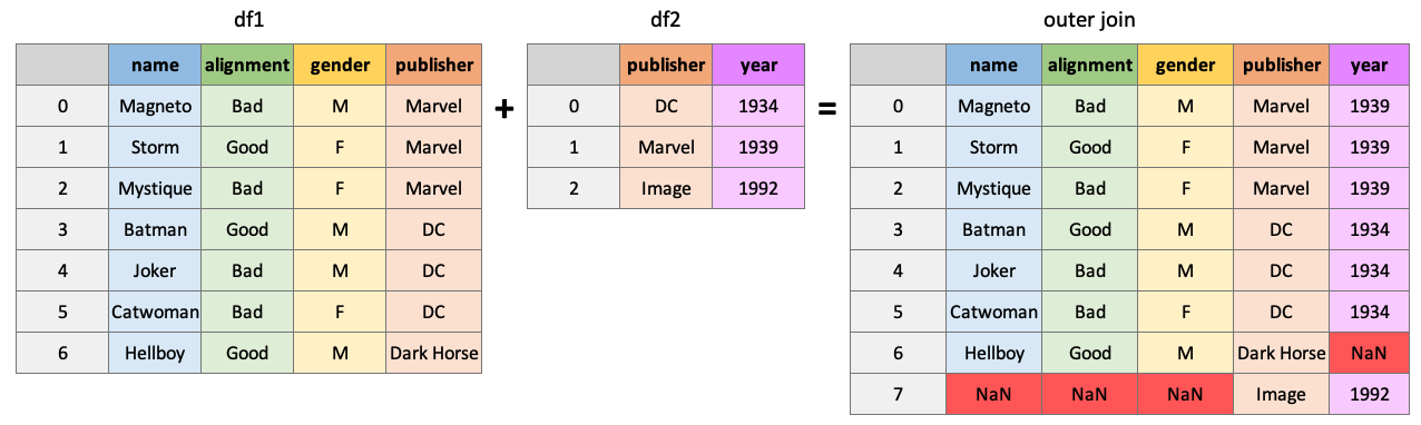
An “outer” join will return all rows of df1 and df2, placing NaNs where information is unavailable:
pd.merge(df1, df2, how="outer", on="publisher")
| name | alignment | gender | publisher | year_founded | |
|---|---|---|---|---|---|
| 0 | Magneto | bad | male | Marvel | 1939.0 |
| 1 | Storm | good | female | Marvel | 1939.0 |
| 2 | Mystique | bad | female | Marvel | 1939.0 |
| 3 | Batman | good | male | DC | 1934.0 |
| 4 | Joker | bad | male | DC | 1934.0 |
| 5 | Catwoman | bad | female | DC | 1934.0 |
| 6 | Hellboy | good | male | Dark Horse Comics | NaN |
| 7 | NaN | NaN | NaN | Image | 1992.0 |
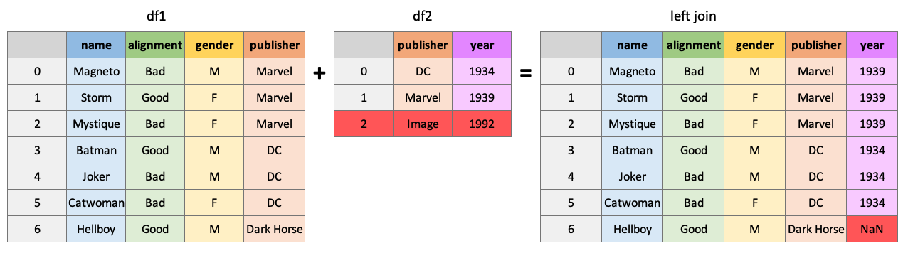
Return all rows from df1 and all columns of df1 and df2, populated where matches occur:
pd.merge(df1, df2, how="left", on="publisher")
| name | alignment | gender | publisher | year_founded | |
|---|---|---|---|---|---|
| 0 | Magneto | bad | male | Marvel | 1939.0 |
| 1 | Storm | good | female | Marvel | 1939.0 |
| 2 | Mystique | bad | female | Marvel | 1939.0 |
| 3 | Batman | good | male | DC | 1934.0 |
| 4 | Joker | bad | male | DC | 1934.0 |
| 5 | Catwoman | bad | female | DC | 1934.0 |
| 6 | Hellboy | good | male | Dark Horse Comics | NaN |
pd.merge(df1, df2, how="right", on="publisher")
| name | alignment | gender | publisher | year_founded | |
|---|---|---|---|---|---|
| 0 | Batman | good | male | DC | 1934 |
| 1 | Joker | bad | male | DC | 1934 |
| 2 | Catwoman | bad | female | DC | 1934 |
| 3 | Magneto | bad | male | Marvel | 1939 |
| 4 | Storm | good | female | Marvel | 1939 |
| 5 | Mystique | bad | female | Marvel | 1939 |
| 6 | NaN | NaN | NaN | Image | 1992 |
There are many ways to specify the key to join dataframes on, you can join on index values, different, column names, etc. Another helpful argument is the indicator argument which will add a column to the result telling you where matches were found in the dataframes:
pd.merge(df1, df2, how="outer", on="publisher", indicator=True)
| name | alignment | gender | publisher | year_founded | _merge | |
|---|---|---|---|---|---|---|
| 0 | Magneto | bad | male | Marvel | 1939.0 | both |
| 1 | Storm | good | female | Marvel | 1939.0 | both |
| 2 | Mystique | bad | female | Marvel | 1939.0 | both |
| 3 | Batman | good | male | DC | 1934.0 | both |
| 4 | Joker | bad | male | DC | 1934.0 | both |
| 5 | Catwoman | bad | female | DC | 1934.0 | both |
| 6 | Hellboy | good | male | Dark Horse Comics | NaN | left_only |
| 7 | NaN | NaN | NaN | Image | 1992.0 | right_only |
By the way, you can use pd.concat() to do a simple “inner” or “outer” join on multiple datadrames at once. It’s less flexible than merge, but can be useful sometimes.
5. More DataFrame Operations
Applying Custom Functions
There will be times when you want to apply a function that is not built-in to Pandas. For this, we also have methods:
df.apply(), applies a function column-wise or row-wise across a dataframe (the function must be able to accept/return an array)df.applymap(), applies a function element-wise (for functions that accept/return single values at a time)series.apply()/series.map(), same as above but for Pandas series
For example, say you want to use a numpy function on a column in your dataframe:
df = pd.read_csv('data/cycling_data.csv')
df[['Time', 'Distance']].apply(np.sin)
| Time | Distance | |
|---|---|---|
| 0 | -0.901866 | 0.053604 |
| 1 | -0.901697 | 0.447197 |
| 2 | -0.035549 | -0.046354 |
| 3 | -0.739059 | 0.270228 |
| 4 | -0.236515 | -0.086263 |
| ... | ... | ... |
| 28 | -0.683372 | 0.063586 |
| 29 | 0.150056 | 0.133232 |
| 30 | 0.026702 | 0.023627 |
| 31 | -0.008640 | 0.221770 |
| 32 | 0.897861 | -0.700695 |
33 rows × 2 columns
Or you may want to apply your own custom function:
def seconds_to_hours(x):
    return x / 3600

df[['Time']].apply(seconds_to_hours)
| Time | |
|---|---|
| 0 | 0.578889 |
| 1 | 0.703056 |
| 2 | 0.517500 |
| 3 | 0.608889 |
| 4 | 0.525278 |
| ... | ... |
| 28 | 0.519444 |
| 29 | 0.596944 |
| 30 | 0.511389 |
| 31 | 0.684167 |
| 32 | 0.511944 |
33 rows × 1 columns
This may have been better as a lambda function…
df[['Time']].apply(lambda x: x / 3600)
| Time | |
|---|---|
| 0 | 0.578889 |
| 1 | 0.703056 |
| 2 | 0.517500 |
| 3 | 0.608889 |
| 4 | 0.525278 |
| ... | ... |
| 28 | 0.519444 |
| 29 | 0.596944 |
| 30 | 0.511389 |
| 31 | 0.684167 |
| 32 | 0.511944 |
33 rows × 1 columns
You can even use functions that require additional arguments. Just specify the arguments in .apply():
def convert_seconds(x, to="hours"):
    if to == "hours":
        return x / 3600
    elif to == "minutes":
        return x / 60

df[['Time']].apply(convert_seconds, to="minutes")
| Time | |
|---|---|
| 0 | 34.733333 |
| 1 | 42.183333 |
| 2 | 31.050000 |
| 3 | 36.533333 |
| 4 | 31.516667 |
| ... | ... |
| 28 | 31.166667 |
| 29 | 35.816667 |
| 30 | 30.683333 |
| 31 | 41.050000 |
| 32 | 30.716667 |
33 rows × 1 columns
Some functions only accept/return a scalar:
int(3.141)
3
float([3.141, 10.345])
---------------------------------------------------------------------------
TypeError                                 Traceback (most recent call last)
<ipython-input-62-97f9c30c3ff1> in <module>
----> 1 float([3.141, 10.345])

TypeError: float() argument must be a string or a number, not 'list'
For these, we need .applymap():
df[['Time']].applymap(int)
| Time | |
|---|---|
| 0 | 2084 |
| 1 | 2531 |
| 2 | 1863 |
| 3 | 2192 |
| 4 | 1891 |
| ... | ... |
| 28 | 1870 |
| 29 | 2149 |
| 30 | 1841 |
| 31 | 2463 |
| 32 | 1843 |
33 rows × 1 columns
However, there are often “vectorized” versions of common functions like this already available, which are much faster. In the case above, we can use .astype() to change the dtype of a whole column quickly:
time_applymap = %timeit  -q -o -r 3 df[['Time']].applymap(float)
time_builtin = %timeit  -q -o -r 3 df[['Time']].astype(float)
print(f"'astype' is {time_applymap.average / time_builtin.average:.2f} faster than 'applymap'!")
'astype' is 1.99 faster than 'applymap'!
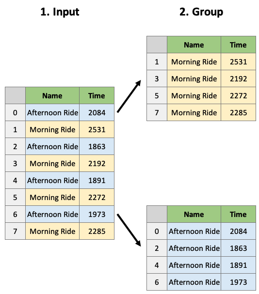
Grouping
Often we are interested in examining specific groups in our data. df.groupby() allows us to group our data based on a variable(s).
df = pd.read_csv('data/cycling_data.csv')
df
| Date | Name | Type | Time | Distance | Comments | |
|---|---|---|---|---|---|---|
| 0 | 10 Sep 2019, 00:13:04 | Afternoon Ride | Ride | 2084 | 12.62 | Rain |
| 1 | 10 Sep 2019, 13:52:18 | Morning Ride | Ride | 2531 | 13.03 | rain |
| 2 | 11 Sep 2019, 00:23:50 | Afternoon Ride | Ride | 1863 | 12.52 | Wet road but nice weather |
| 3 | 11 Sep 2019, 14:06:19 | Morning Ride | Ride | 2192 | 12.84 | Stopped for photo of sunrise |
| 4 | 12 Sep 2019, 00:28:05 | Afternoon Ride | Ride | 1891 | 12.48 | Tired by the end of the week |
| ... | ... | ... | ... | ... | ... | ... |
| 28 | 4 Oct 2019, 01:08:08 | Afternoon Ride | Ride | 1870 | 12.63 | Very tired, riding into the wind |
| 29 | 9 Oct 2019, 13:55:40 | Morning Ride | Ride | 2149 | 12.70 | Really cold! But feeling good |
| 30 | 10 Oct 2019, 00:10:31 | Afternoon Ride | Ride | 1841 | 12.59 | Feeling good after a holiday break! |
| 31 | 10 Oct 2019, 13:47:14 | Morning Ride | Ride | 2463 | 12.79 | Stopped for photo of sunrise |
| 32 | 11 Oct 2019, 00:16:57 | Afternoon Ride | Ride | 1843 | 11.79 | Bike feeling tight, needs an oil and pump |
33 rows × 6 columns
Let’s group this dataframe on the column Name:
dfg = df.groupby(by='Name')
dfg
<pandas.core.groupby.generic.DataFrameGroupBy object at 0x112491050>
What is a DataFrameGroupBy object? It contains information about the groups of the dataframe:
The groupby object is really just a dictionary of index-mappings, which we could look at if we wanted to:
dfg.groups
{'Afternoon Ride': [0, 2, 4, 6, 9, 10, 12, 14, 16, 18, 20, 22, 24, 26, 28, 30, 32], 'Morning Ride': [1, 3, 5, 7, 8, 11, 13, 15, 17, 19, 21, 23, 25, 27, 29, 31]}
We can also access a group using the .get_group() method:
dfg.get_group('Afternoon Ride')
| Date | Name | Type | Time | Distance | Comments | |
|---|---|---|---|---|---|---|
| 0 | 10 Sep 2019, 00:13:04 | Afternoon Ride | Ride | 2084 | 12.62 | Rain |
| 2 | 11 Sep 2019, 00:23:50 | Afternoon Ride | Ride | 1863 | 12.52 | Wet road but nice weather |
| 4 | 12 Sep 2019, 00:28:05 | Afternoon Ride | Ride | 1891 | 12.48 | Tired by the end of the week |
| 6 | 17 Sep 2019, 00:15:47 | Afternoon Ride | Ride | 1973 | 12.45 | Legs feeling strong! |
| 9 | 18 Sep 2019, 00:15:52 | Afternoon Ride | Ride | 2101 | 12.48 | Pumped up tires |
| 10 | 19 Sep 2019, 00:30:01 | Afternoon Ride | Ride | 48062 | 12.48 | Feeling good |
| 12 | 20 Sep 2019, 01:02:05 | Afternoon Ride | Ride | 2961 | 12.81 | Feeling good |
| 14 | 24 Sep 2019, 00:35:42 | Afternoon Ride | Ride | 2076 | 12.47 | Oiled chain, bike feels smooth |
| 16 | 25 Sep 2019, 00:07:21 | Afternoon Ride | Ride | 1775 | 12.10 | Feeling really tired |
| 18 | 26 Sep 2019, 00:13:33 | Afternoon Ride | Ride | 1860 | 12.52 | raining |
| 20 | 27 Sep 2019, 01:00:18 | Afternoon Ride | Ride | 1712 | 12.47 | Tired by the end of the week |
| 22 | 1 Oct 2019, 00:15:07 | Afternoon Ride | Ride | 1732 | NaN | Legs feeling strong! |
| 24 | 2 Oct 2019, 00:13:09 | Afternoon Ride | Ride | 1756 | NaN | A little tired today but good weather |
| 26 | 3 Oct 2019, 00:45:22 | Afternoon Ride | Ride | 1724 | 12.52 | Feeling good |
| 28 | 4 Oct 2019, 01:08:08 | Afternoon Ride | Ride | 1870 | 12.63 | Very tired, riding into the wind |
| 30 | 10 Oct 2019, 00:10:31 | Afternoon Ride | Ride | 1841 | 12.59 | Feeling good after a holiday break! |
| 32 | 11 Oct 2019, 00:16:57 | Afternoon Ride | Ride | 1843 | 11.79 | Bike feeling tight, needs an oil and pump |
The usual thing to do however, is to apply aggregate functions to the groupby object:
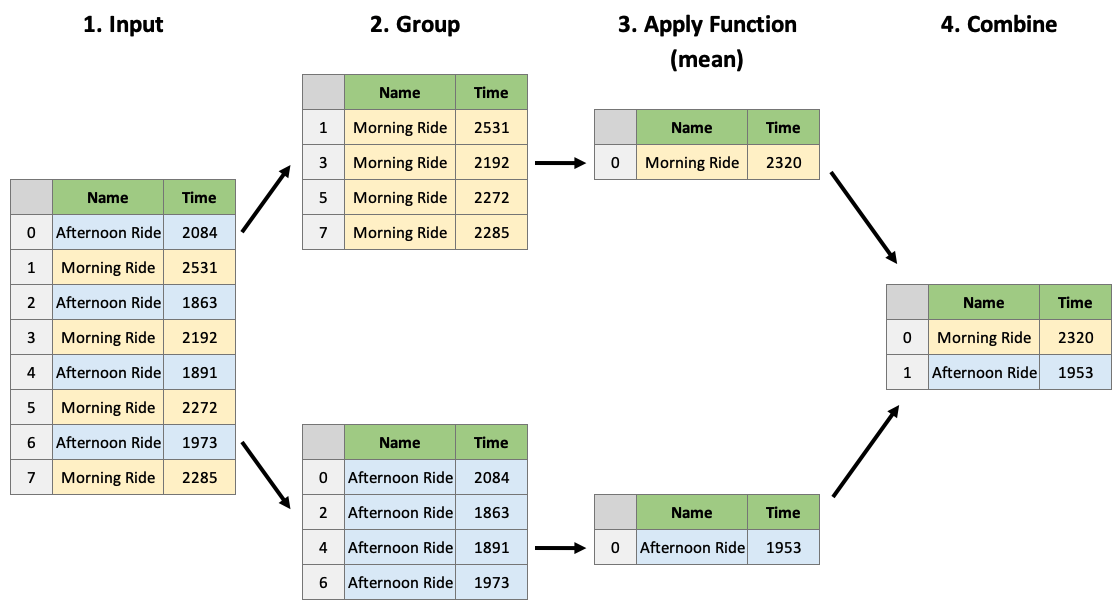
dfg.mean()
| Time | Distance | |
|---|---|---|
| Name | ||
| Afternoon Ride | 4654.352941 | 12.462 |
| Morning Ride | 2299.875000 | 12.860 |
We can apply multiple functions using .aggregate():
dfg.aggregate(['mean', 'sum', 'count'])
| Time | Distance | |||||
|---|---|---|---|---|---|---|
| mean | sum | count | mean | sum | count | |
| Name | ||||||
| Afternoon Ride | 4654.352941 | 79124 | 17 | 12.462 | 186.93 | 15 |
| Morning Ride | 2299.875000 | 36798 | 16 | 12.860 | 205.76 | 16 |
And even apply different functions to different columns:
def num_range(x):
    return x.max() - x.min()

dfg.aggregate({"Time": ['max', 'min', 'mean', num_range],
               "Distance": ['sum']})
| Time | Distance | ||||
|---|---|---|---|---|---|
| max | min | mean | num_range | sum | |
| Name | |||||
| Afternoon Ride | 48062 | 1712 | 4654.352941 | 46350 | 186.93 |
| Morning Ride | 2903 | 2090 | 2299.875000 | 813 | 205.76 |
By the way, you can use aggregate for non-grouped dataframes too. This is pretty much what df.describe does under-the-hood:
df.agg(['mean', 'min', 'count', num_range])
| Date | Name | Type | Time | Distance | Comments | |
|---|---|---|---|---|---|---|
| min | 1 Oct 2019, 00:15:07 | Afternoon Ride | Ride | 1712.000000 | 11.790000 | A little tired today but good weather |
| count | 33 | 33 | 33 | 33.000000 | 31.000000 | 33 |
| mean | NaN | NaN | NaN | 3512.787879 | 12.667419 | NaN |
| num_range | NaN | NaN | NaN | 46350.000000 | 2.780000 | NaN |
Dealing with Missing Values
Missing values are typically denoted with NaN. We can use df.isnull() to find missing values in a dataframe. It returns a boolean for each element in the dataframe:
df.isnull()
| Date | Name | Type | Time | Distance | Comments | |
|---|---|---|---|---|---|---|
| 0 | False | False | False | False | False | False |
| 1 | False | False | False | False | False | False |
| 2 | False | False | False | False | False | False |
| 3 | False | False | False | False | False | False |
| 4 | False | False | False | False | False | False |
| ... | ... | ... | ... | ... | ... | ... |
| 28 | False | False | False | False | False | False |
| 29 | False | False | False | False | False | False |
| 30 | False | False | False | False | False | False |
| 31 | False | False | False | False | False | False |
| 32 | False | False | False | False | False | False |
33 rows × 6 columns
But it’s usually more helpful to get this information by row or by column using the .any() or .info() method:
df.info()
<class 'pandas.core.frame.DataFrame'>
RangeIndex: 33 entries, 0 to 32
Data columns (total 6 columns):
 #   Column    Non-Null Count  Dtype
---  ------    --------------  -----
 0   Date      33 non-null     object
 1   Name      33 non-null     object
 2   Type      33 non-null     object
 3   Time      33 non-null     int64
 4   Distance  31 non-null     float64
 5   Comments  33 non-null     object
dtypes: float64(1), int64(1), object(4)
memory usage: 1.7+ KB
df[df.isnull().any(axis=1)]
| Date | Name | Type | Time | Distance | Comments | |
|---|---|---|---|---|---|---|
| 22 | 1 Oct 2019, 00:15:07 | Afternoon Ride | Ride | 1732 | NaN | Legs feeling strong! |
| 24 | 2 Oct 2019, 00:13:09 | Afternoon Ride | Ride | 1756 | NaN | A little tired today but good weather |
When you have missing values, we usually either drop them or impute them.You can drop missing values with df.dropna():
df.dropna()
| Date | Name | Type | Time | Distance | Comments | |
|---|---|---|---|---|---|---|
| 0 | 10 Sep 2019, 00:13:04 | Afternoon Ride | Ride | 2084 | 12.62 | Rain |
| 1 | 10 Sep 2019, 13:52:18 | Morning Ride | Ride | 2531 | 13.03 | rain |
| 2 | 11 Sep 2019, 00:23:50 | Afternoon Ride | Ride | 1863 | 12.52 | Wet road but nice weather |
| 3 | 11 Sep 2019, 14:06:19 | Morning Ride | Ride | 2192 | 12.84 | Stopped for photo of sunrise |
| 4 | 12 Sep 2019, 00:28:05 | Afternoon Ride | Ride | 1891 | 12.48 | Tired by the end of the week |
| ... | ... | ... | ... | ... | ... | ... |
| 28 | 4 Oct 2019, 01:08:08 | Afternoon Ride | Ride | 1870 | 12.63 | Very tired, riding into the wind |
| 29 | 9 Oct 2019, 13:55:40 | Morning Ride | Ride | 2149 | 12.70 | Really cold! But feeling good |
| 30 | 10 Oct 2019, 00:10:31 | Afternoon Ride | Ride | 1841 | 12.59 | Feeling good after a holiday break! |
| 31 | 10 Oct 2019, 13:47:14 | Morning Ride | Ride | 2463 | 12.79 | Stopped for photo of sunrise |
| 32 | 11 Oct 2019, 00:16:57 | Afternoon Ride | Ride | 1843 | 11.79 | Bike feeling tight, needs an oil and pump |
31 rows × 6 columns
Or you can impute (“fill”) them using .fillna(). This method has various options for filling, you can use a fixed value, the mean of the column, the previous non-nan value, etc:
df = pd.DataFrame([[np.nan, 2, np.nan, 0],
                   [3, 4, np.nan, 1],
                   [np.nan, np.nan, np.nan, 5],
                   [np.nan, 3, np.nan, 4]],
                  columns=list('ABCD'))
df
| A | B | C | D | |
|---|---|---|---|---|
| 0 | NaN | 2.0 | NaN | 0 |
| 1 | 3.0 | 4.0 | NaN | 1 |
| 2 | NaN | NaN | NaN | 5 |
| 3 | NaN | 3.0 | NaN | 4 |
df.fillna(0) # fill with 0
| A | B | C | D | |
|---|---|---|---|---|
| 0 | 0.0 | 2.0 | 0.0 | 0 |
| 1 | 3.0 | 4.0 | 0.0 | 1 |
| 2 | 0.0 | 0.0 | 0.0 | 5 |
| 3 | 0.0 | 3.0 | 0.0 | 4 |
df.fillna(df.mean()) # fill with the mean
| A | B | C | D | |
|---|---|---|---|---|
| 0 | 3.0 | 2.0 | NaN | 0 |
| 1 | 3.0 | 4.0 | NaN | 1 |
| 2 | 3.0 | 3.0 | NaN | 5 |
| 3 | 3.0 | 3.0 | NaN | 4 |
df.fillna(method='bfill') # backward (upwards) fill from non-nan values
| A | B | C | D | |
|---|---|---|---|---|
| 0 | 3.0 | 2.0 | NaN | 0 |
| 1 | 3.0 | 4.0 | NaN | 1 |
| 2 | NaN | 3.0 | NaN | 5 |
| 3 | NaN | 3.0 | NaN | 4 |
df.fillna(method='ffill') # forward (downward) fill from non-nan values
| A | B | C | D | |
|---|---|---|---|---|
| 0 | NaN | 2.0 | NaN | 0 |
| 1 | 3.0 | 4.0 | NaN | 1 |
| 2 | 3.0 | 4.0 | NaN | 5 |
| 3 | 3.0 | 3.0 | NaN | 4 |
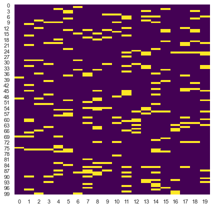
Finally, sometimes I use visualizations to help identify (patterns in) missing values. One thing I often do is print a heatmap of my dataframe to get a feel for where my missing values are. If you want to run this code, you may need to install seaborn:
conda install seaborn
import seaborn as sns
sns.set(rc={'figure.figsize':(7, 7)})
df
| A | B | C | D | |
|---|---|---|---|---|
| 0 | NaN | 2.0 | NaN | 0 |
| 1 | 3.0 | 4.0 | NaN | 1 |
| 2 | NaN | NaN | NaN | 5 |
| 3 | NaN | 3.0 | NaN | 4 |
sns.heatmap(df.isnull(), cmap='viridis', cbar=False);

# Generate a larger synthetic dataset for demonstration
np.random.seed(2020)
npx = np.zeros((100,20))
mask = np.random.choice([True, False], npx.shape, p=[.1, .9])
npx[mask] = np.nan
sns.heatmap(pd.DataFrame(npx).isnull(), cmap='viridis', cbar=False);