
Chapter 4: Training Neural Networks
By Tomas Beuzen 🚀

Chapter Outline
Chapter Learning Objectives
Explain how backpropagation works at a high level.
Describe the difference between training loss and validation loss when creating a neural network.
Identify and describe common techniques to avoid overfitting/apply regularization to neural networks, e.g., early stopping, drop out, L2 regularization.
Use
PyTorchto develop a fully-connected neural network and training pipeline.
Imports
import numpy as np
import pandas as pd
import torch
from torch import nn
from torchvision import transforms, datasets, utils
from torch.utils.data import DataLoader, TensorDataset
from utils.plotting import *
1. Differentiation, Backpropagation, Autograd
In previous chapters we’ve discussed optimization algorithms like gradient descent, stochastic gradient descent, ADAM, etc. These algorithms need the gradient of the loss function w.r.t the model parameters to optimize the parameters:
We’ve been able to calculate the gradient by hand for things like linear regression and logistic regression. But how would you work out the gradient for this very simple network for regression:
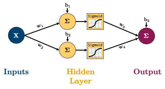
The equation for calculating the output of that network is below, it’s the linear layers and activation functions (Sigmoid in this case) recursively stuck together:
So how would we calculate the gradient of say the MSE loss w.r.t to all our parameters?
We have 3 options:
Symbolic differentiation: i.e., “do it by hand” like we learned in calculus.
Numerical differentiation: for example, approximating the derivative using finite differences \(\frac{df(x)}{dx} \approx \frac{f(x+h)-f(x)}{h}\).
Automatic differentiation: the “best of both worlds”.
We’ll be looking at option 3 Automatic Differentiation (AD) here, as we use a particular flavour of AD called “backpropagation” to train neural networks. But if you’re interested in learning more about the other methods, see Appendix C: Computing Derivatives.
1.1. Backpropagation
Backpropagation is the algorithm we use to compute the gradients needed to train the parameters of a neural network. In backpropagation, the main idea is to decompose our network into smaller operations with simple, codeable derivatives. We then combine all these smaller operations together with the chain rule. The term “backpropagation” stems from the fact that we start at the end of our network and then propagate backwards. I’m going to go through a short example based on this network:
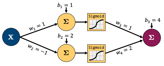
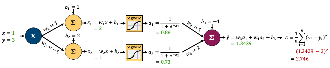
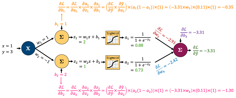
Let’s decompose that into smaller operations. I’ve introduced some new variables to hold intermediate states \(z_i\) (node output before activation) and \(a_i\) (node output after activation). I’ll also feed in one sample data point (x, y) = (1, 3) and am showing intermediate outputs in green and the final loss in red. This is called the “forward pass” step - where I feed in data and calculate outputs from left to right:
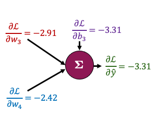
Now let’s zoom in to the outpout node and calculate the gradients for just the parameters connected to that node. It looks complicated but the derivatives are very simple - take some time to examine this figure and you’ll see!
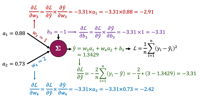
That all boils down to this:
Now, the beauty of backpropagation is that we can use these results to easily calculate derivatives earlier in the network using the chain rule. I’ll do that for \(b_1\) and \(b_2\) below. Once again, it looks complicated, but we’re simply combining a bunch of small, simple derivatives with the chain rule:
I’ve left calculating the gradients of \(w_1\) and \(w_2\) up to you. All the gradients for the network boil down to this:
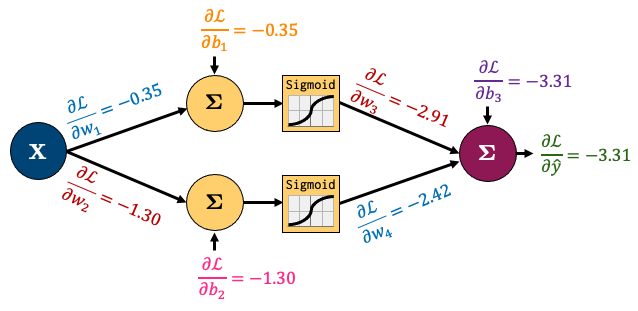
So summarising the process:
We “forward pass” some data through our network
We “backpropagate” the error through the network to calculate gradients
Luckily, you’ll never do this by hand again, because torch.autograd does all this for us!
1.2. Autograd
torch.autograd is PyTorch’s automatic differentiation engine which helps us implement backpropagation. In plain English: torch.autograd automatically calculates and stores derivatives for your network. Consider our simple network above:
class network(torch.nn.Module):
    def __init__(self, input_size, hidden_size, output_size):
        super().__init__()
        self.hidden = torch.nn.Linear(input_size, hidden_size)
        self.output = torch.nn.Linear(hidden_size, output_size)

    def forward(self, x):
        x = self.hidden(x)
        x = torch.sigmoid(x)
        x = self.output(x)
        return x
model = network(1, 2, 1)  # make an instance of our network
model.state_dict()['hidden.weight'][:] = torch.tensor([[1], [-1]])  # fix the weights manually based on the earlier figure
model.state_dict()['hidden.bias'][:] = torch.tensor([1, 2])
model.state_dict()['output.weight'][:] = torch.tensor([[1, 2]])
model.state_dict()['output.bias'][:] = torch.tensor([-1])
x, y = torch.tensor([1.0]), torch.tensor([3.0])  # our x, y data
Now let’s check the gradient of the bias of the output node:
print(model.output.bias.grad)
None
It’s currently None!
PyTorch is tracking the operations in our network and how to calculate the gradient (more on that a bit later), but it hasn’t calculated anything yet because we don’t have a loss function and we haven’t done a forward pass to calculate the loss so there’s nothing to backpropagate yet!
Let’s define a loss now:
criterion = torch.nn.MSELoss()
Now we can force Pytorch to “backpropagate” the errors, like we just did by hand earlier by:
Doing a “forward pass” of our
(x, y)data and calculating theloss;“Backpropagating” the loss by calling
loss.backward()
loss = criterion(model(x), y)
loss.backward()  # backpropagates the error to calculate gradients!
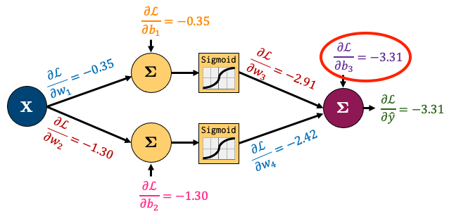
Now let’s check the gradient of the bias of the output node (\(\frac{\partial \mathscr{L}}{\partial b_3}\)):
print(model.output.bias.grad)
tensor([-3.3142])
It matches what we calculated earlier!
That is just so fantastic! In fact, we can make sure that all our gradients match what we calculated by hand:
print("Hidden Layer Gradients")
print("Bias:", model.hidden.bias.grad)
print("Weights:", model.hidden.weight.grad.squeeze())
print()
print("Output Layer Gradients")
print("Bias:", model.output.bias.grad)
print("Weights:", model.output.weight.grad.squeeze())
Hidden Layer Gradients
Bias: tensor([-0.3480, -1.3032])
Weights: tensor([-0.3480, -1.3032])

Output Layer Gradients
Bias: tensor([-3.3142])
Weights: tensor([-2.9191, -2.4229])
Now that we have the gradients, what’s the next step? We use our optimization algorithm to update our weights! These are our current weights:
model.state_dict()
OrderedDict([('hidden.weight',
              tensor([[ 1.],
                      [-1.]])),
             ('hidden.bias', tensor([1., 2.])),
             ('output.weight', tensor([[1., 2.]])),
             ('output.bias', tensor([-1.]))])
To optimize them, we:
Define an
optimizer;Ask it to update our weights based on our gradients using
optimizer.step().
optimizer = torch.optim.SGD(model.parameters(), lr=0.1)
optimizer.step()
Our weights should now be different:
model.state_dict()
OrderedDict([('hidden.weight',
              tensor([[ 1.0348],
                      [-0.8697]])),
             ('hidden.bias', tensor([1.0348, 2.1303])),
             ('output.weight', tensor([[1.2919, 2.2423]])),
             ('output.bias', tensor([-0.6686]))])
Amazing!
One last thing for you to know: Pytorch does not automatically clear the gradients after using them. So if I call loss.backward() again, my gradients accumulate:
optimizer.zero_grad()  # <- I'll explain this in the next cell
for _ in range(1, 6):
    loss = criterion(model(x), y)
    loss.backward()
    print(f"b3 gradient after call {_} of loss.backward():", model.hidden.bias.grad)
b3 gradient after call 1 of loss.backward(): tensor([-0.1991, -0.5976])
b3 gradient after call 2 of loss.backward(): tensor([-0.3983, -1.1953])
b3 gradient after call 3 of loss.backward(): tensor([-0.5974, -1.7929])
b3 gradient after call 4 of loss.backward(): tensor([-0.7966, -2.3906])
b3 gradient after call 5 of loss.backward(): tensor([-0.9957, -2.9882])
Our gradients are accumulating each time we call loss.backward()! So we need to tell Pytorch to “zero the gradients” each iteration using optimizer.zero_grad():
for _ in range(1, 6):
    optimizer.zero_grad()  # <- don't forget this!!!
    loss = criterion(model(x), y)
    loss.backward()
    print(f"b3 gradient after call {_} of loss.backward():", model.hidden.bias.grad)
b3 gradient after call 1 of loss.backward(): tensor([-0.1991, -0.5976])
b3 gradient after call 2 of loss.backward(): tensor([-0.1991, -0.5976])
b3 gradient after call 3 of loss.backward(): tensor([-0.1991, -0.5976])
b3 gradient after call 4 of loss.backward(): tensor([-0.1991, -0.5976])
b3 gradient after call 5 of loss.backward(): tensor([-0.1991, -0.5976])
Note: you might wonder why PyTorch behaves like this. Well, there are some cases we might want to accumulate the gradient. For example, if we want to calculate the gradients over several batches before updating our weights. But don’t worry about that for now - most of the time, you’ll want to be “zeroing out” the gradients each iteration.
1.3. Computational Graph (Optional)
PyTorch’s autograd basically keeps a record of our data and network operations in a computational graph. That’s beyond the scope of this chapter, but if you’re interested in learning more, I recommend this excellent video. Also, torchviz is a useful package to look at the “computational graph” PyTorch is building for us under the hood:
from torchviz import make_dot
make_dot(model(torch.rand(1, 1)))

2. Training Neural Networks
The big takeaway from the last section is that PyTorch’s autograd takes care of the gradients for us. We just need to put all the pieces together properly. Remember the below trainer() function I used last chapter to train my network. Now we know what all this means!
def trainer(model, criterion, optimizer, dataloader, epochs=5):
    """Simple training wrapper for PyTorch network."""

    train_loss = []
    for epoch in range(epochs):  # for each epoch
        losses = 0
        for X, y in dataloader:  # for each batch
            optimizer.zero_grad()       # Zero all the gradients w.r.t. parameters
            y_hat = model(X).flatten()  # Forward pass to get output
            loss = criterion(y_hat, y)  # Calculate loss based on output
            loss.backward()             # Calculate gradients w.r.t. parameters
            optimizer.step()            # Update parameters
            losses += loss.item()       # Add loss for this batch to running total
        train_loss.append(losses / len(dataloader))  # loss = total loss in epoch / number of batches = loss per batch
    return train_loss
Notice how I calculate the loss for each epoch by summing up the loss for each batch in that epoch? I then divide the loss per epoch by total number of batches to get the average loss per batch in an epoch (I store that loss in running_losses).
Dividing by the number of batches “decouples” our loss from the batch size. So if I run another experiment with a different batch size, I’ll still be able to compare losses for that experiment with this one. We’ll explore this concept more later.
If our model is being trained correctly, our loss should go down over time. Let’s try it out with some sample data:
# Create dataset
torch.manual_seed(0)
X = torch.arange(-3, 3, 0.15)
y = X ** 2 + X * torch.normal(0, 1, (40,))
dataloader = DataLoader(TensorDataset(X[:, None], y), batch_size=1, shuffle=True)
plot_regression(X, y, y_range=[-1, 10], dy=1)
model = network(1, 3, 1)
criterion = torch.nn.MSELoss()
optimizer = torch.optim.Adam(model.parameters(), 0.1)
train_loss = trainer(model, criterion, optimizer, dataloader, epochs=101)
plot_regression(X, y, model(X[:, None]).detach(), y_range=[-1, 10], dy=1)
The model looks like a good fit, so presumably the loss went down as epochs progressed, let’s take a look:
plot_loss(train_loss)
2.1. Validation Loss
We’ve been focussing on training loss so far, but as we know, we need to validate our model on new “unseen” data! For this, we’ll need some validation data, I’m going to split our dataset in half to create a trainloader and a validloader:
# Create dataset
torch.manual_seed(0)
X_valid = torch.arange(-3.0, 3.0)
y_valid = X_valid ** 2
trainloader = DataLoader(TensorDataset(X, y), batch_size=1, shuffle=True)
validloader = DataLoader(TensorDataset(X_valid, y_valid), batch_size=1, shuffle=True)
Now the wonderful thing about PyTorch is that you are in full control - you can do whatever you want! So here, after each epoch, I’m going to record the validation loss by looping over my validation batches, it’s just a little extra module I add to my training function:
def trainer(model, criterion, optimizer, trainloader, validloader, epochs=5):
    """Simple training wrapper for PyTorch network."""

    train_loss = []
    valid_loss = []
    for epoch in range(epochs):  # for each epoch
        train_batch_loss = 0
        valid_batch_loss = 0

        # Training
        model.train()  # This puts the model in "training mode", this is the default mode.
                       # We'll use a different mode, "evaluation mode", for validation.
        for X, y in trainloader:
            optimizer.zero_grad()       # Zero all the gradients w.r.t. parameters
            y_hat = model(X).flatten()  # Forward pass to get output
            loss = criterion(y_hat, y)  # Calculate loss based on output
            loss.backward()             # Calculate gradients w.r.t. parameters
            optimizer.step()            # Update parameters
            train_batch_loss += loss.item()  # Add loss for this batch to running total
        train_loss.append(train_batch_loss / len(trainloader))  # loss = total loss in epoch / number of batches = loss per batch

        # Validation
        model.train()  # This puts the model in "evaluation mode". It's important to do this when our model
                       # includes some randomness like dropout layers which we'll see later. It turns off
                       # this randomness for validation purposes.
        with torch.no_grad():  # this stops pytorch doing computational graph stuff under-the-hood and saves memory and time
            for X_valid, y_valid in validloader:
                y_hat = model(X_valid).flatten()  # Forward pass to get output
                loss = criterion(y_hat, y_valid)  # Calculate loss based on output
                valid_batch_loss += loss.item()   # Add loss for this batch to running total


        valid_loss.append(valid_batch_loss / len(validloader))
    return train_loss, valid_loss
model = network(1, 6, 1)
criterion = torch.nn.MSELoss()
optimizer = torch.optim.Adam(model.parameters(), lr=0.05)
train_loss, valid_loss = trainer(model, criterion, optimizer, trainloader, validloader, epochs=201)
plot_loss(train_loss, valid_loss)
What do we see above? Well, we’re obviously overfitting (fitting to closely to the training data such that we do poorly on the validation data). We are optimizing too well! One way we could avoid overfitting is by terminating the training if our validation loss starts going up, this is called “early stopping”.
2.2. Early stopping
Early stopping is a way of avoiding overfitting. As training progresses, if we notice the validation loss increasing (while the training loss decreases), that’s usually an indication of overfitting. The validation loss may go up and down from epoch to epoch, so usually we define a “patience” which is a number of consecutive epochs we’re willing to allow the validation loss to increase before we stop. Once again, the beauty of PyTorch is how easy it is to customize your network in this way:
def trainer(model, criterion, optimizer, trainloader, validloader, epochs=5, patience=5):
    """Simple training wrapper for PyTorch network."""

    train_loss = []
    valid_loss = []
    for epoch in range(epochs):  # for each epoch
        train_batch_loss = 0
        valid_batch_loss = 0

        # Training
        for X, y in trainloader:
            optimizer.zero_grad()       # Zero all the gradients w.r.t. parameters
            y_hat = model(X).flatten()  # Forward pass to get output
            loss = criterion(y_hat, y)  # Calculate loss based on output
            loss.backward()             # Calculate gradients w.r.t. parameters
            optimizer.step()            # Update parameters
            train_batch_loss += loss.item()  # Add loss for this batch to running total
        train_loss.append(train_batch_loss / len(trainloader))  # loss = total loss in epoch / number of batches = loss per batch

        # Validation
        with torch.no_grad():  # this stops pytorch doing computational graph stuff under-the-hood and saves memory and time
            for X_valid, y_valid in validloader:
                y_hat = model(X_valid).flatten()  # Forward pass to get output
                loss = criterion(y_hat, y_valid)  # Calculate loss based on output
                valid_batch_loss += loss.item()   # Add loss for this batch to running total

        valid_loss.append(valid_batch_loss / len(validloader))

        # Early stopping
        if epoch > 0 and valid_loss[-1] > valid_loss[-2]:
            consec_increases += 1
        else:
            consec_increases = 0
        if consec_increases == patience:
            print(f"Stopped early at epoch {epoch + 1} - val loss increased for {consec_increases} consecutive epochs!")
            break

    return train_loss, valid_loss
model = network(1, 6, 1)
criterion = torch.nn.MSELoss()
optimizer = torch.optim.Adam(model.parameters(), lr=0.05)
train_loss, valid_loss = trainer(model, criterion, optimizer, trainloader, validloader, epochs=201, patience=3)
plot_loss(train_loss, valid_loss)
Stopped early at epoch 58 - val loss increased for 3 consecutive epochs!
There are more advanced implementations of early stopping out there, but you get the idea!
3. Regularization
Recall that regularization is a technique to help avoid overfitting. There are many regularization techniques available in neural networks. I’ll discuss the two main ones here:
Drop out
L2 regularization
3.1. Drop Out
Drop out is a common regularization technique and is very simple. Basically, each iteration, we randomly chose some nodes in a layer and don’t update their weights (to do this we set the output of the nodes to 0). A simple example:
dropout_layer = torch.nn.Dropout(p=0.5)  # 50% probability that a node will be set to 0 ("dropped out")
inputs = torch.randn(5, 3)
inputs
tensor([[ 0.8693, -2.1287,  0.6825],
        [-0.8968, -0.4331, -0.4829],
        [-1.8682, -1.0257,  0.5033],
        [ 1.5761,  1.8840, -1.2248],
        [-1.4531,  0.3420, -1.1799]])
dropout_layer(inputs)
tensor([[ 1.7386, -0.0000,  1.3651],
        [-1.7936, -0.0000, -0.0000],
        [-0.0000, -0.0000,  0.0000],
        [ 0.0000,  0.0000, -2.4496],
        [-2.9063,  0.6840, -2.3598]])
In the above, note how about 50% of nodes have been given a value of 0!
3.2. L2 Regularization
Recall that in L2 we had this penalty to the loss: \(\frac{\lambda}{2}||w||^2\). \(\lambda\) is the regularization parameter. L2 regularization is called “weight-decay” in PyTorch (because we are coercing the weights to be smaller I suppose). It’s an argument in most optimizers which you can specify:
torch.optim.Adam(model.parameters(), lr=0.1, weight_decay=0.5) # here weight_decay is λ in the above equation
Adam (
Parameter Group 0
    amsgrad: False
    betas: (0.9, 0.999)
    eps: 1e-08
    lr: 0.1
    weight_decay: 0.5
)
4. Putting it all Together with Bitmojis
Here I thought we’d put everything we learned in this chapter together to predict some bitmojis. I have a folder of images with the following structure:
data
└── bitmoji_bw
    ├── train
    │   ├── not_tom
    │   └── tom
    └── valid
        ├── not_tom
        └── tom
TRAIN_DIR = "data/bitmoji_bw/train/"
VALID_DIR = "data/bitmoji_bw/valid/"
IMAGE_SIZE = 50
BATCH_SIZE = 32

data_transforms = transforms.Compose([
    transforms.Resize(IMAGE_SIZE),
    transforms.Grayscale(num_output_channels=1),
    transforms.ToTensor()
])
# Training data
train_dataset = datasets.ImageFolder(root=TRAIN_DIR, transform=data_transforms)
train_loader = torch.utils.data.DataLoader(train_dataset, batch_size=BATCH_SIZE, shuffle=True)
# Validation data
valid_dataset = datasets.ImageFolder(root=VALID_DIR, transform=data_transforms)
valid_loader = torch.utils.data.DataLoader(valid_dataset, batch_size=BATCH_SIZE, shuffle=True)
sample_batch = next(iter(train_loader))
plot_bitmojis(sample_batch)

Now to the network. I’m going to make a function linear_block() to help create my network and keep things DRY:
def linear_block(input_size, output_size):
    return nn.Sequential(
        nn.Linear(input_size, output_size),
        nn.LeakyReLU(),
        nn.Dropout(0.1)
    )

class BitmojiClassifier(nn.Module):
    def __init__(self, input_size):
        super().__init__()
        self.main = nn.Sequential(
            linear_block(input_size, 256),
            linear_block(256, 128),
            linear_block(128, 64),
            linear_block(64, 16),
            nn.Linear(16, 1)
        )

    def forward(self, x):
        out = self.main(x)
        return out
Now the training function. This is getting long but it’s just all the bits we’ve seen before!
def trainer(model, criterion, optimizer, trainloader, validloader, epochs=5, patience=5, verbose=True):
    """Simple training wrapper for PyTorch network."""

    train_loss = []
    valid_loss = []
    train_accuracy = []
    valid_accuracy = []
    for epoch in range(epochs):  # for each epoch
        train_batch_loss = 0
        train_batch_acc = 0
        valid_batch_loss = 0
        valid_batch_acc = 0

        # Training
        for X, y in trainloader:
            optimizer.zero_grad()       # Zero all the gradients w.r.t. parameters
            y_hat = model(X.view(X.shape[0], -1)).flatten()  # Forward pass to get output
            y_hat_labels = torch.sigmoid(y_hat) > 0.5        # convert probabilities to False (0) and True (1)
            loss = criterion(y_hat, y.type(torch.float32))   # Calculate loss based on output
            loss.backward()             # Calculate gradients w.r.t. parameters
            optimizer.step()            # Update parameters
            train_batch_loss += loss.item()  # Add loss for this batch to running total
            train_batch_acc += (y_hat_labels == y).type(torch.float32).mean().item()   # Average accuracy for this batch
        train_loss.append(train_batch_loss / len(trainloader))     # loss = total loss in epoch / number of batches = loss per batch
        train_accuracy.append(train_batch_acc / len(trainloader))  # accuracy

        # Validation
        model.eval()  # this turns off those random dropout layers, we don't want them for validation!
        with torch.no_grad():  # this stops pytorch doing computational graph stuff under-the-hood and saves memory and time
            for X, y in validloader:
                y_hat = model(X.view(X.shape[0], -1)).flatten()  # Forward pass to get output
                y_hat_labels = torch.sigmoid(y_hat) > 0.5        # convert probabilities to False (0) and True (1)
                loss = criterion(y_hat, y.type(torch.float32))   # Calculate loss based on output
                valid_batch_loss += loss.item()                  # Add loss for this batch to running total
                valid_batch_acc += (y_hat_labels == y).type(torch.float32).mean().item()   # Average accuracy for this batch
        valid_loss.append(valid_batch_loss / len(validloader))
        valid_accuracy.append(valid_batch_acc / len(validloader))  # accuracy
        model.train()  # turn back on the dropout layers for the next training loop

        # Print progress
        if verbose:
            print(f"Epoch {epoch + 1}:",
                  f"Train Loss: {train_loss[-1]:.3f}.",
                  f"Valid Loss: {valid_loss[-1]:.3f}.",
                  f"Train Accuracy: {train_accuracy[-1]:.2f}.",
                  f"Valid Accuracy: {valid_accuracy[-1]:.2f}.")

        # Early stopping
        if epoch > 0 and valid_loss[-1] > valid_loss[-2]:
            consec_increases += 1
        else:
            consec_increases = 0
        if consec_increases == patience:
            print(f"Stopped early at epoch {epoch + 1} - val loss increased for {consec_increases} consecutive epochs!")
            break

    results = {"train_loss": train_loss,
               "valid_loss": valid_loss,
               "train_accuracy": train_accuracy,
               "valid_accuracy": valid_accuracy}
    return results
Let’s do it!
model = BitmojiClassifier(IMAGE_SIZE * IMAGE_SIZE)
criterion = nn.BCEWithLogitsLoss()
optimizer = torch.optim.Adam(model.parameters())
results = trainer(model, criterion, optimizer, train_loader, valid_loader, epochs=20, patience=3)
Epoch 1: Train Loss: 0.697. Valid Loss: 0.693. Train Accuracy: 0.48. Valid Accuracy: 0.49.
Epoch 2: Train Loss: 0.694. Valid Loss: 0.694. Train Accuracy: 0.50. Valid Accuracy: 0.50.
Epoch 3: Train Loss: 0.693. Valid Loss: 0.693. Train Accuracy: 0.50. Valid Accuracy: 0.48.
Epoch 4: Train Loss: 0.692. Valid Loss: 0.693. Train Accuracy: 0.52. Valid Accuracy: 0.50.
Epoch 5: Train Loss: 0.693. Valid Loss: 0.693. Train Accuracy: 0.51. Valid Accuracy: 0.51.
Epoch 6: Train Loss: 0.692. Valid Loss: 0.691. Train Accuracy: 0.52. Valid Accuracy: 0.52.
Epoch 7: Train Loss: 0.694. Valid Loss: 0.693. Train Accuracy: 0.50. Valid Accuracy: 0.50.
Epoch 8: Train Loss: 0.692. Valid Loss: 0.689. Train Accuracy: 0.54. Valid Accuracy: 0.56.
Epoch 9: Train Loss: 0.691. Valid Loss: 0.690. Train Accuracy: 0.52. Valid Accuracy: 0.57.
Epoch 10: Train Loss: 0.683. Valid Loss: 0.682. Train Accuracy: 0.57. Valid Accuracy: 0.56.
Epoch 11: Train Loss: 0.693. Valid Loss: 0.693. Train Accuracy: 0.53. Valid Accuracy: 0.52.
Epoch 12: Train Loss: 0.685. Valid Loss: 0.683. Train Accuracy: 0.56. Valid Accuracy: 0.54.
Epoch 13: Train Loss: 0.677. Valid Loss: 0.678. Train Accuracy: 0.59. Valid Accuracy: 0.58.
Epoch 14: Train Loss: 0.668. Valid Loss: 0.665. Train Accuracy: 0.61. Valid Accuracy: 0.61.
Epoch 15: Train Loss: 0.664. Valid Loss: 0.654. Train Accuracy: 0.61. Valid Accuracy: 0.62.
Epoch 16: Train Loss: 0.668. Valid Loss: 0.682. Train Accuracy: 0.60. Valid Accuracy: 0.56.
Epoch 17: Train Loss: 0.681. Valid Loss: 0.685. Train Accuracy: 0.56. Valid Accuracy: 0.55.
Epoch 18: Train Loss: 0.677. Valid Loss: 0.654. Train Accuracy: 0.58. Valid Accuracy: 0.63.
Epoch 19: Train Loss: 0.665. Valid Loss: 0.667. Train Accuracy: 0.61. Valid Accuracy: 0.60.
Epoch 20: Train Loss: 0.654. Valid Loss: 0.651. Train Accuracy: 0.62. Valid Accuracy: 0.65.
Epoch 21: Train Loss: 0.664. Valid Loss: 0.655. Train Accuracy: 0.61. Valid Accuracy: 0.62.
Epoch 22: Train Loss: 0.658. Valid Loss: 0.652. Train Accuracy: 0.61. Valid Accuracy: 0.63.
Epoch 23: Train Loss: 0.652. Valid Loss: 0.643. Train Accuracy: 0.62. Valid Accuracy: 0.65.
Epoch 24: Train Loss: 0.653. Valid Loss: 0.621. Train Accuracy: 0.61. Valid Accuracy: 0.66.
Epoch 25: Train Loss: 0.653. Valid Loss: 0.641. Train Accuracy: 0.63. Valid Accuracy: 0.66.
Epoch 26: Train Loss: 0.647. Valid Loss: 0.635. Train Accuracy: 0.61. Valid Accuracy: 0.65.
Epoch 27: Train Loss: 0.644. Valid Loss: 0.680. Train Accuracy: 0.62. Valid Accuracy: 0.54.
Epoch 28: Train Loss: 0.642. Valid Loss: 0.625. Train Accuracy: 0.63. Valid Accuracy: 0.65.
Epoch 29: Train Loss: 0.627. Valid Loss: 0.648. Train Accuracy: 0.66. Valid Accuracy: 0.65.
Epoch 30: Train Loss: 0.650. Valid Loss: 0.660. Train Accuracy: 0.63. Valid Accuracy: 0.58.
plot_loss(results["train_loss"], results["valid_loss"], results["train_accuracy"], results["valid_accuracy"])
I couldn’t get very good accuracy with this model and there’s a reason for that - we’re not considering the structure in our image. We’re flattening our images down into independent pixels, but the relationship between pixels is probably important! We’ll exploit that next chapter when we get to CNNs. For now, let’s try a random image for fun:
image = torch.from_numpy(plt.imread("img/tom.png"))
image = transforms.Resize(IMAGE_SIZE)(image[None, None, :, :])
prediction = model(image.view(1, -1))   # Flatten image to shape (1, 784) and predict it
prediction = torch.sigmoid(prediction)  # Coerce predictions to probabilities
label = int(prediction > 0.5)           # Get class label - 1 if propbability > 0.5, else 0
plot_bitmoji(image, label)

Well, at least we got that one!