Multivariate Normal Distributions
A simple explanation and example of the multivariate normal distribution.
Introduction
Multivariate distribution are used when there is correlation between your variables: i.e., the value of one variable affects the value of the other(s). I always found multivariate distributions a difficult concept to understand. One of the simplest multivariate distributions is the multivariate normal distribution, the focus of this short post. The multivariate normal distribution really clicked for me when a friend gave me a very intuitive analogy which I’ll be using throughout this post.
Imagine you want to measure two variables: your heart rate at 9:00am, and your heart rate at 9:05am in beats per minute (bpm). There is likely correlation between these two variables, i.e., your heart rate at 9:05am is probably pretty similar to your heart rate at 9:00am. You measure this data for 7 days, and you get the following data:
import numpy as np
import pandas as pd
import plotly.graph_objects as go
from scipy.stats import norm, multivariate_normal
np.random.seed(2020)
pd.options.plotting.backend = "plotly"
df = pd.DataFrame({"9:00": [60, 70, 45, 55, 61, 57, 64],
                   "9:05": [62, 69, 45, 60, 62, 60, 67]})
df
| 9:00 | 9:05 | |
|---|---|---|
| 0 | 60 | 62 |
| 1 | 70 | 69 |
| 2 | 45 | 45 |
| 3 | 55 | 60 |
| 4 | 61 | 62 |
| 5 | 57 | 60 |
| 6 | 64 | 67 |
While we’re here let’s check the correlation in our data (we’ll use this later on):
df.corr()
| 9:00 | 9:05 | |
|---|---|---|
| 9:00 | 1.000000 | 0.965826 |
| 9:05 | 0.965826 | 1.000000 |
There’s a strong positive correlation here, indicating that the two variables do appear to be related. In the next few sections, I’ll use the above data to build up to an intuition of the multivariate normal distribution.
Univariate Normal Distribution
Let’s start by exploring the univariate (one variable) normal distribution. One thing you could do with the data above is model each variable as two independent univariate normal distributions, which are each defined by two parameters: the mean μ and the standard deviation σ. Let’s fit the two distributions now:
mu_900, std_900 = norm.fit(df['9:00'])
mu_905, std_905 = norm.fit(df['9:05'])
Now that we have two univariate distributions, let’s randomly draw 7 observations from them to simulate a week of new data:
pd.DataFrame({"9:00": norm.rvs(mu_900, std_900, size=7).astype(int),
              "9:05": norm.rvs(mu_905, std_905, size=7).astype(int)})
| 9:00 | 9:05 | |
|---|---|---|
| 0 | 46 | 61 |
| 1 | 59 | 63 |
| 2 | 50 | 56 |
| 3 | 54 | 54 |
| 4 | 52 | 70 |
| 5 | 49 | 69 |
| 6 | 58 | 52 |
Notice anything strange? The heart rate measured at 9:00am is sometimes very different to the heart rate at 9:05am. By simulating our two variables as univariate normal distributions, there is no “sharing of information” between the variables, i.e., they are independent and don’t influence each other (although they probably should). Here are the two distributions for your reference:
x = np.linspace(40, 80, 100)
df_uvn = pd.DataFrame({"9:00": norm.pdf(x, mu_900, std_900),
                       "9:05": norm.pdf(x, mu_905, std_905)})
fig = df_uvn.plot(width=700, height=400, title="Univariate Normal Heart Rate Distributions")
fig.update_xaxes(title_text='Heart Rate')
fig.update_yaxes(title_text='Probability Density')
fig.update_layout(xaxis = dict(range=[0, 100], tickmode = 'linear', dtick = 20),
                  yaxis = dict(range=[0, 0.06], tickmode = 'linear', dtick = 0.01))
Multivariate Normal Distribution
We could more realistically model our heart rate data as a multivariate distribution, which will include the correlation between the variables we noticed earlier. I’m going to let scipy formulate the multivariate normal distribution for me and I’ll directly draw 7 observations from it:
pd.DataFrame(multivariate_normal.rvs(df.mean(), df.cov(), size=7).astype(int),
             columns=["9:00", "9:05"])
| 9:00 | 9:05 | |
|---|---|---|
| 0 | 57 | 56 |
| 1 | 62 | 62 |
| 2 | 55 | 57 |
| 3 | 42 | 44 |
| 4 | 59 | 60 |
| 5 | 60 | 60 |
| 6 | 71 | 70 |
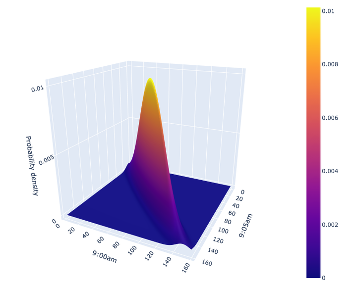
Ah, much better, our simulated data is much closer to reality now than what we had previously with our univariate distributions. It’s a bit harder to plot this as we are now working in 3D (two dimensions for the variables, one for the probability density) but let’s give it a go:
x1, x2 = np.mgrid[40:80:0.25, 40:80:0.25]
z = multivariate_normal(df.mean(), df.cov()).pdf(np.dstack((x1, x2)))
fig = go.Figure(data=[go.Surface(z=z)])
fig.update_xaxes(title_text='Heart Rate')
fig.update_yaxes(title_text='Probability Density')
fig.update_layout(width=700, height=700, title="Multivariate Normal Heart Rate Distribution",
                  scene = dict(xaxis = dict(title = '9:05am'),
                               yaxis = dict(title = '9:00am'),
                               zaxis = dict(title = 'Probability density')),
                  margin=dict(l=0, r=50, b=50, t=50))
Feel free to move the above plot around with your cursor. You can interpret the “height/elevation” in the plot as a probability, i.e., the higher the elevation, the more likely the values of heart rate at 9:00am/9:05am. In particular, note how if we observe a heart rate of 60 at 9:00am, the most probably value of your heart rate at 9:05am is about 62 or so. We can confirm that by looking at the cross-section of the above plot at 9:00am = 60:
fig = pd.DataFrame(z[80,:], index=x1[:,80]).plot(width=700, height=400, title="Heart Rate at 9:05am given that Heart Rate at 9:00am = 60bpm")
fig.update_xaxes(title_text='Heart Rate')
fig.update_yaxes(title_text='Probability Density')
fig.update_layout(xaxis = dict(range=[40, 80], tickmode = 'linear', dtick = 5),
                  showlegend=False)
Summary
I hope this short post helped give some intuition about what multivariate distributions are and why they are useful. The example above is actually a bivariate distribution (two variables), but the intuition provided extends to more than two variables - it just gets harder to plot in more dimensions so I stuck to two variables here!